IEG 환경지질연구정보센터

1. Introduction

The analysis of land cover is a key in land-use plans, and land cover is closely connected with various human/physical phenomena. The study and interpretation of land covers requires much detail for the

understanding of the underlying processes. However, it is difficult to get accurate data about land cover features due to both the necessary manual activity and statistical analysis of large data sets. Nevertheless, it becomes a common knowledge that land cover classification can be greatly facilitated by the use of remotely sensed data

Integration of Multi-spectral Remote Sensing Images and GIS Thematic Data for

Supervised Land Cover Classification

Dong-Ho Jang* and Chung, Chang-Jo F**

National Research Laboratory (Harmful Algal Blooming Control), Kongju National University*

Geological Survey of Canada**

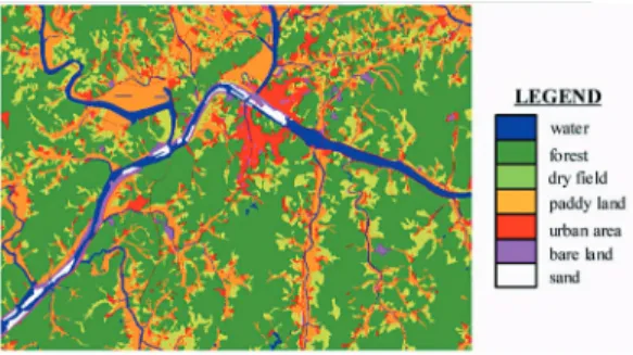
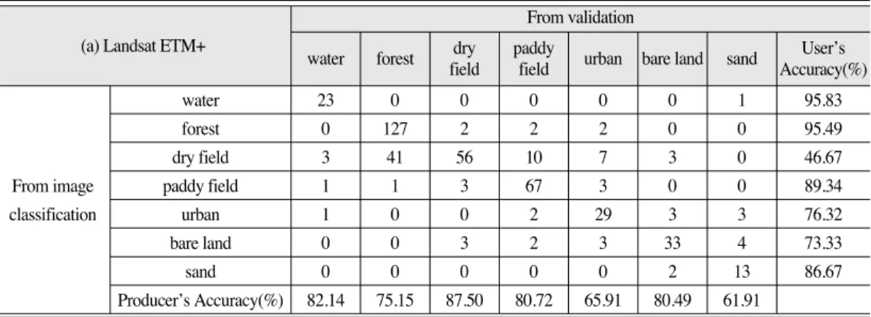
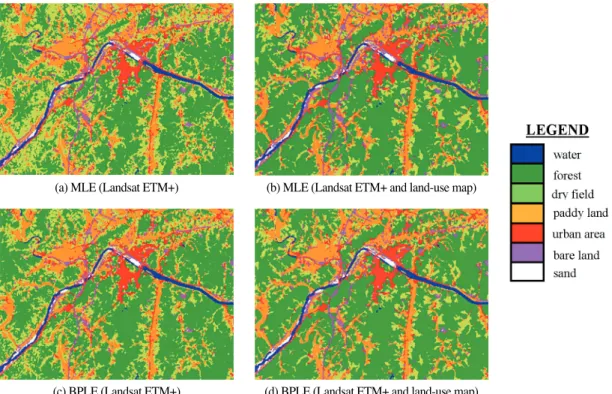
Abstract : Nowadays, interests in land cover classification using not only multi-sensor images but also thematic GIS information are increasing. Often, although useful GIS information for the classification is available, the traditional MLE (maximum likelihood estimation techniques) does not allow us to use the information, due to the fact that it cannot handle the GIS data properly. This paper propose two extended MLE algorithms that can integrate both remote sensing images and GIS thematic data for land- cover classification. They include modified MLE and Bayesian predictive likelihood estimation technique (BPLE) techniques that can handle both categorical GIS thematic data and remote sensing images in an integrated manner. The proposed algorithms were evaluated through supervised land-cover classification with Landsat ETM+ images and an existing land-use map in the Gongju area, Korea. As a result, the proposed method showed considerable improvements in classification accuracy, when compared with other multi-spectral classification techniques. The integration of remote sensing images and the land-use map showed that overall accuracy indicated an improvement in classification accuracy of 10.8% when using MLE, and 9.6% for the BPLE. The case study also showed that the proposed algorithms enable the extraction of the area with land-cover change. In conclusion, land cover classification results produced through the integration of various GIS spatial data and multi-spectral images, will be useful to involve complementary data to make more accurate decisions.

Key Words : Land Cover Classification, Maximum Likelihood Estimation, Bayesian Predictive Likelihood Estimation, Classification Accuracy.

Received 24 August 2004; Accepted 16 September 2004.

owing to their wide area coverage, synchronism, periodicity and economical efficiency.

To perform land cover classification, the integration of data from multi-sources data including remote sensing images and GIS thematic information can be utilized to reduce the classification error obtained by single-source classification. Conventional parametric classification methods require that the multi-spectral data be described by a common statistical model. Such the models cannot be easily established for combining different data types, e.g., spectral data from remote sensing image and categorical data from a GIS. Another problem with the conventional approach is that the different data sources might not be equally reliable. The development of an appropriate model for the classification of data from multi-sources and different numeric mode (e.g., a mixture of continuous and categorical data) is essential for land cover classification.

Several new methodologies for multi-source integration in land cover classification have been proposed in the recent years. In a methodological point of view, they include the Bayesian probabilistic approach (Solberg et al., 1996; Tso and Mather, 1999;

Warrender and Augusteijn, 1999), the neural networks (Serpico et al., 1996; Benediktsson and Sveinsson, 1997; Dai and Khorram, 1999), fuzzy sets (Solaiman et al., 1999) and evidence theory (Peddle, 1995; Peddle and Ferguson, 2002; Franklin et al., 2002). These studies include land cover classification: the development of new land cover classification techniques through the integration of multi-sensor/source remote sensing images, and the accuracy verification of these techniques (Solberg, 1999).

Only a limited set of studies have involved contextual multi-source classification. Richards et al. (1982) extended the methods used for spatial contextual classification based on probabilistic relaxation to incorporate ancillary data. Binaghi et al. (1997) presented a knowledge-based framework for con-textual

classification based on fuzzy set theory. Wan and Fraser (1994) used multiple self-organizing maps for contextual classification. Le H’ egarat-Mascle et al.

(1997) combined the use of a Markov random field model with Dempster-Shafer theory. Smits and Dellepiane (1997) used a multichannel image segmentation method based on Markov random fields with adaptive neighborhoods.

In relation to the use of categorical data in the classification of remote sensing data, Solberg et al.

(1996) proposed a Markov Random Field model for the classification of multisource data including Landsat TM images, ERS-1 SAR images, and categorical GIS ground cover data. Solberg (1999) also proposed a methodology for forest map revision by using a Markov Random Field Model, an existing forest map and remote sensing data.

Also, recent progress in data acquisition technology has enabled the simultaneous use of high-resolution remote sensing images and GIS-based thematic maps.

These all techniques, in tern, require a new analytical method that is capable of synchronous analysis of GIS multi-source data.

In this paper, we have extended the Maximum Likelihood Estimation technique (MLE) to accommodate both remote sensing imageries and GIS data for land cover classification. MLE is based on the assumption that the distribution function of remote sensing images of each land cover class is normal distribution with known parameters, the mean vector and the variance-covariance matrix (Press, 1972).

However, in practice, although the normality

assumption of the distribution functions is reasonable, it

is not possible to assume that we know the mean vectors

and the variance-covariance matrices of the distribution

functions. In reality, these parameters are estimated from

the input database. When the parameters are estimated

from the data, theoretically MLE is not a right procedure

(Press, 1972; McLallen, 1990) and the proper procedure

is Bayesian predictive likelihood estimation technique (BPLE). If there are small samples, it is known that BPLE shows better performance than that from MLE.

While, for large samples, the performance between BPLE and MLE is similar.

We also have extended BPLE to handle both remote sensing images and GIS categorical data. The accuracy of this classification integration technique was verified by comparisons made with actual-measured validation data. The proposed procedure was evaluated using Landsat ETM+ images and an existing land-use maps, in the Gongju-si, in Korea.

2. Methodologies

1) Basic idea

Consider r land cover types to be constructed using a classification method in a study area. We will use k layers of categorized data layers and h layers of remotely sensed image data layers for the classification.

We also assume that we have sufficient training data which is available for each land cover type in the study area. For a pixel p, let (x

, …, x

, y

, …, y

) denote pixels values at p where the first k values, x

, …, x

correspond to the categorical data layers and subsequent h values, y

, …, y

represent the continuous data layers.

P{M

| x

, …, x

, y

, …, y

}, (i = 1, …, r) (1) As usual, let denote the conditional probability that the pixel p belongs to the i

class, M

given that (x

, …, x

, y

, …, y

) are pixels values at p. Often, the probability in (1) is also called “posterior” probability meaning that it is the probability that p belongs to M

after observing k+h pixel values, (x

, …, x

, y

, …, y

) at p.

If we know how to compute P{M

| x

, …, x

, y

, …, y

} for every class i (i = 1, …, r) for a given pixel p with (x

, …, x

, y

, …, y

), then the classification problem becomes very simple, in that, we assign the pixel p to

the class g, if P{M

| x

, …, x

, y

, …, y

} is the largest among all P{M

| x

, …, x

, y

, …, y

} (i = 1, …, r).

Using Bayes’ theorem (Richards, 1995), we express the probability in (1) in the following form:

P{M

| x

, …, x

, y

, …, y

} =

, (2)

where P{M

} is the “prior” probability that the pixel p belongs to the i

class, M

before observing (x

, …, x

, y

, …, y

) at p and it contrasts to the posterior probability in (1) and

P{x

, …, x

, y

, …, y

} =

P{x

, …, x

, y

, …, y

| M

}P{M

}. (3)

There are several ways to estimate P{M

| x

, …, x

, y

, …, y

}, (i = 1, …, r) from the training data. Instead of estimating P{M

| x

, …, x

, y

, …, y

} directly in (1), we can try to obtain it by estimating, equivalently, P{x

, …, x

, y

, …, y

| M

} and P{M

} from the training data by using (2). Consider P{x

, …, x

, y

, …, y

| M

}, the conditional probability that the pixel p has (x

, …, x

, y

, …, y

) observations, assuming that the pixel p comes from the i

class, M

. In other words, it is the k+h multivariate frequency distribution function of the pixel values in the M

. Therefore, to estimate the posterior probability in (1) is equivalent to estimating the frequency distribution functions of the pixel values in r classes using the training data. The frequency distribution function of the class, M

is usually expressed as f{x

, …, x

, y

, …, y

| M

} instead of P{x

, …, x

, y

, …, y

| M

}.

2) Separation of categorized data layers and continuous data layers

To handle the multivariate frequency distribution functions of two different types of data layers, we have made the following assumption of conditional independence:

S

P{x

, …, x

, y

, …, y

| M

}P{M

}

P{x

, …, x

, y

, …, y

}

f{x

, …, x

, y

, …, y

| M

} =

f{x

, …, x

| M

} f{y

, …, y

| M

}, (i = 1, …, r). (4) Under the assumption of (4), the k + h dimensional multivariate frequency distribution function, f{x

, …, x

, y

, …, y

| M

} is expressed as a multiple of the k dimensional multivariate discrete distribution function for the categorical data and the h dimensional multivariate continuous distribution function for the continuous data and hence we will estimate the frequency distribution function as a multiple of two distribution functions, one for categorical data layers and the other for continuous data layers.

Under most practical circumstances, the conditional independent assumption in (4) is reasonable except for some of the categorized data layers were directly deducted from the continuous data layers

3) Estimation of frequency distribution function for categorized data layers

Among r frequency distribution functions, consider one f{x

, …, x

| M

} for a pixel p with k pixel values (x

, …, x

), each x

representing a category in the j

data layer where the pixel p belongs to M

class. f{x

, …, x

| M

} is the m

x m

x … x m

cross-classified contingency table, where mj represents the number of categories in the j

layer. The x

x x

x … x x

cell of the k-dimensional table represents the number of M

class pixels that belongs to x

category in the 1

layer, x

category in the 2

layer and x

category in the k

layer. Let us denote U

…

as the unique condition sub-area (Chung et al., 1995; Clerici et al., 2002) with the classes, x

, …, x

and the pixels in the sub-area belong to the x

category in the 1

layer, the x

category in the 2

layer and the x

category in the k

layer. # of M

class pixels within U

…

is the x

x x

x … x x

cell of the k-dimensional table.

The first non-parametric estimate of f{x

, …, x

| M

} is the empirical frequency distribution function from the

training data:

˘f{x

, …, x

| M

} =

# of M

class pixels within U

…

from the

training data. (5)

However, if we assume that f{x

, …, x

| M

} is the multivariate multinomial frequency distribution functions (Johnson and Kotz, 1972). Then, the maximum likelihood estimate of this multinomial distribution function is the empirical k-dimensional contingency table in (5). Although it is simple to compute, but we strongly suggest NOT using the estimate in (5), when the number of categorized data layers is more than two.

The second procedure to estimate f{x

, …, x

| M

}, (i

= 1, …, r) assumes, as in (4), that the k categorical layers are conditionally independent and hence, we have:

f{x

, …, x

| M

} = f{x

| M

} … f{x

| M

}, (i = 1, …, r).(6) Instead of considering all the k layers at the same time, we may estimate the distribution function as a multiple of k separate distribution functions. Each separate function is estimated by the empirical frequency distribution function using each single categorical data layer:

˜f{x

| M

} = # of M

class pixels within x

category

within the j

layer (7)

Using (6) and (7) under the conditional independence assumption, we obtain an empirical estimate of f{x

, …, x

| M

} by:

˜f{x

, …, x

| M

} = ˜f{x

| M

} … ˜f{x

| M

}, (i = 1, …, r).(8)

As before, if we assume that f{x

, …, x

| M

} is the

multivariate multinomial frequency distribution

functions and the conditional independence in (6), then,

the empirical frequency function in (8) is also the

maximum likelihood estimate of f{x

, …, x

| M

}. We

strongly recommend the use of equation (8) rather than

(5), when the number of categorized data layers is more

than two. When the number is greater than two and the

number of the classes in each layer is more than five, then the sizes of many of the unique condition sub-areas become very small and consequently many of the ˘f{x

,

…, x

| M

} are equal to zero. When we integrate the zero value with the estimate of the frequency distribution function from the continuous data layers, they generate an undesirable negative impact on the classification maps.

4) Estimation of frequency distribution function for continuous data layers

Consider the frequency distribution function for continuous data layers, f{y

, …, y

| M

} for a pixel p with h pixel values (y

, …, y

), where each y

represents a real value at y within the j

continuous data layer. The simplest non-parametric estimate for the function is an empirical frequency distribution function based on either histogram or kernel method. When the number of layers is more than two, then such empirical distribution is not recommended as an estimate. The next non-parametric procedure requires conditional independence as in (4).

We assume that the h continuous layers are conditionally independent and hence, we have:

f{y

, …, y

| M

} = f{y

| M

} … f{y

| M

}, (i = 1, …, r).(9) Instead of considering k-dimensional multivariate distribution functions, we may estimate the frequency distribution function as a multiple of k separate univariate frequency distribution functions, where each univeriate individual distribution is estimated by an empirical frequency distribution:

¨f{y

, …, y

| M

} = ¨f{y

| M

} … ¨f{y

| M

}, (i = 1, …, r).(10) In many situations, the estimate in (7) is an effective estimate of f{y

, …, y

| M

}. A parametric estimate of f{y

, …, y

| M

} is obtained by assuming that it is the multivariate normal distribution functions, N(m

, S

) where m

and S

are the k-dimensional mean vectors for M

class and the k x k dimensional covariance

matrix for M

, respectively. Suppose that ˆ m

and ˆS

are the sample mean vector and the sample covariance matrix computed from the training data, then they are the maximum likelihood estimates of m

and S

(Hubert-Moy et al., 2001). Using this MLE (Richards, 1995), we obtain the following estimate:

…

f{y

, …, y

| M

} =

exp {

^(y

^{m ˆ}

^{) ’ ˆS}

^(y

^{m ˆ}

⁾ } ^{, (11)}

where y = (y

, …, y

) is an h-dimensional vector containing h observed values and the computation operations in (11) are vector and matrix calculations.

However, as discussed in Press (1972), instead of the normal distribution with the sample mean vector and the sample covariance matrix in (11), the proper distribution function under the normal assumption with the sample mean vector and covariance matrix is the multivariate Student t-distribution function:

˜f{y

, …, y

| M

} =

, (12)

where ˆp

is an estimate of the prior probability, P{M

}. It should be used as an estimate of f{y

, …, y

| M

} instead of one in (11).

If the normality assumptions are reasonably realistic conditions, then we recommend the estimate shown in (12), but the estimate is almost similar to that in (11) of the maximum likelihood estimate. In practice, most of commercial computer packages don’t have a computer program for (12). In this case, we recommend the use of (11) instead of (12) because the values are almost identical. However, if the empirical distribution functions appear to be far from the normality, then we recommend the estimate in (10) under the conditional

1 2 1

2p || ˆS

||

G ( ) ^ˆp

G ( ^N

2

^h ) || ^(N

^{1) ˆS}

||

N

2

[ ^{1 + N}

^N

^{1 (y}

^{m ˆ}

^{)’ ˆS}

^(y

^{m ˆ}

⁾ ]

[ ^(N

^N + 1)p

]

independence assumption.

5) Combining the estimates from categorized and continuous data layers and decision rule

Under the assumption of (13), the k + h dimensional multivariate frequency distribution function, f{x

, …, x

, y

, …, y

| M

} containing both the categorized and continuous data layers can be expressed as a multiple of the discrete distribution function for the categorical data and the continuous distribution function for the continuous data and we have discussed how these estimates could be obtained from the training data. We obtained an estimate of f{x

, …, x

, y

, …, y

| M

} by:

ˆf{x

, …, x

, y

, …, y

| M

} =

ˆf{x

, …, x

| M

} ˆf{y

, …, y

| M

}, (13) where ˆf{x

, …, x

| M

} is obtained by either (5) or (8) and ˆf{y

, …, y

| M

} is obtained by one of (10), (11) and (12). For every pixel with k+h pixel values, (x

,

…, x

, y

, …, y

), we compute ˆf{x

, …, x

, y

, …, y

| M

}, one for each class, i = 1, …, r. Then we assign the pixel p to the class g, if ˆf{x

, …, x

, y

, …, y

| M

} is

the largest among all ˆf{x

, …, x

, y

, …, y

| M

} (i = 1,

…, r).

3. Study area and data collection

This study area covers approximately 247 km

, located at the center of Chungnam province, occupies a basin surrounded by Charyeong Mountains in the northwest and Mt. Gyeryong in the southeast. It lies between 127˚01’00’’and 127˚13’14’’ East of longitude and 36˚22’42’’ and 36˚ 30’01’’ North of latitude(Fig. 1).

A Landsat ETM+ image was acquired on 16 September 2000. This is a very complicated scene due to the great mixture of surface features and also the spatial variability of the land cover. The image was registered to the Transverse Mercator coordinate system using 1:25,000 topographic maps.

A land-use map of the study area was obtained as vector-polygon coverage from the National Geography Institute (Fig. 2). Twenty-one classes are defined in this coverage that including residential, industrial, commercial, agricultural, and natural land uses. The

Fig. 1. Location of the Gongju-si area in Korea (Landsat ETM + image acquired on 16 September 2000).

land-use map was constructed for the year 2000 and was compiled using field survey and aerial photography. The raw data in the land-use map were converted into grid data, so that they could be integrated with the Landsat ETM+ image data. The study area has been subsequently extracted from this converted database and reclassified into the same classes as satellite images.

This reclassified land-use map was then integrated with the Landsat ETM+ image in order to produce a land cover classification map. The main reason for the use of the land-use map is as follows. First, the integration of the existing land-use map with the Landsat ETM+

image can generate the revised land-use map because of the use of the remote sensing data acquired after the land-use map generation. Second, information from the existing land-use map can be regarded as a priori or temporal contextual information for the probabilistic classification of the Landsat ETM+ image.

On the basis of an extensive knowledge of the area and an accurate ground survey carried out during the period of 1999-2000, 7 classes were found to be representative of the land cover, as shown in Table 1.

Defined 7 classes in the study area as follows: “water”,

“forest”, “dry field”, “paddy field”, “urban area”, “bare land” and “sand”.

The training data were extracted from the screen digitizing of digital maps, aerial photography, and ground survey. The same training data were used for comparing different classification techniques. In this

study, a total of 13,615 training data were selected for comparing all the classifiers. These also were used integration to accommodate both Landsat ETM+ and land-use data for land cover classification.

To compute the classification accuracy, a classification error matrix was first prepared and then the accuracy statistics were extracted from it. There is a tendency to overestimate the overall accuracy if the training set area is used in the classification error matrix.

Reference data were collected from the training data and from field survey. We selected places exhibiting uniform spectral characteristics that are evenly located in the study area. The number of reference pixels used for the supervised classification was 450. Reference pixel numbers are shown in Table 1, the pixel numbers are as follows: 28 for “water”, 169 for the “forest”, 64 for the

“dry field”, 83 for the “paddy field”, 44 for the “urban area”, 41 for the “bare land” and 21 for “sand”, respectively.

4. The result of land covers classification using Landsat ETM+ and land-use maps

In this study, MLE and BPLE techniques were applied to multi-spectral classification with Landsat ETM+ information. At the same time, GIS multi-source Table 1. Land cover classes and numbers of training and

validation pixels over the study area.

Class Training pixels Validation pixels

water 1297 28

forest 5684 169

dry field 1097 64

paddy field 2723 83

urban area 1694 44

bare land 908 41

sand 212 21

Total 13615 450

Class Training pixels Validation pixels

Fig. 2. land-use map of the study area.

classification, where Landsat ETM+ images and land- use maps were applied together, was also used.

Table 2 includes all error matrices from integrated algorithms and two individual techniques. To begin with, both the MLE and the BPLE techniques showed similar accuracy in multi-spectral image classification using the Landsat ETM+ image information. Both Tables 2 and 3 have shown that MLE and the BPLE techniques took individually 77.33% and 80.89% of overall accuracy, respectively. In kappa statistic, the MLE and the BPLE techniques were 0.72% and 0.76%, respectively. User’s accuracy exhibited classification accuracy of over 75% for most class categories. Both

“dry field” and “bare land” showed lower accuracy than the other class categories. The MLE and the BPLE

techniques in “dry field” especially revealed 46.67% and 54.00%, respectively, which were the lowest values in classification accuracy. This is due to the similarity in spectral information in “dry field” and “forest” because of the sensor recording in autumn, a seasonal factor.

As to producer’s accuracy, for the MLE and the BPLE techniques, these showed similar classification accuracy. “Bare land” and “sand” represented the low classification accuracy. In “bare land”, the MLE and the BPLE techniques had 80.49% and 68.29%, respectively, while for “sand” both had an accuracy of 61.91% and 71.43%, respectively. This low classification accuracy in sand resulted from the similarity in spectral reflectance of “bare land” with “sand”, which was due to the presence of sand in bare land.

Table 2. Calculated error matrices for the MLE. (a) Landsat ETM+ data. (b) Landsat ETM+ and land-use map.

(a) Landsat ETM+ From validation

water forest dry paddy urban bare land sand User’s

field field Accuracy (%)

water 23 0 0 0 0 0 1 95.83

forest 0 127 2 2 2 0 0 95.49

dry field 3 41 56 10 7 3 0 46.67

From image paddy field 1 1 3 67 3 0 0 89.34

classification urban 1 0 0 2 29 3 3 76.32

bare land 0 0 3 2 3 33 4 73.33

sand 0 0 0 0 0 2 13 86.67

Producer’s Accuracy(%) 82.14 75.15 87.50 80.72 65.91 80.49 61.91 Overall Accuracy = 77.33%, Overall Kappa Statistic = 0.716%

(b) Landsat ETM+ andLand-use maps From validation

water forest dry paddy urban bare land sandUser’s Accuracy (%)

field field

water 24 0 0 0 0 0 0 100.0

forest 0 165 10 1 0 1 0 93.22

dry field 1 2 50 3 5 1 0 80.65

From image paddy field 2 2 1 74 3 0 0 90.24

classification urban 1 0 0 2 35 4 0 83.33

bare land 0 0 3 3 1 33 6 71.74

sand 0 0 0 0 0 2 15 88.24

Producer’s Accuracy(%) 85.71 97.63 78.12 89.16 79.55 80.49 71.43 Overall Accuracy = 88.00%, Overall Kappa Statistic = 0.845%

From validation (a) Landsat ETM+

water forest dry paddy

urban bare land sand User’s

field field Accuracy(%)

From validation (b) Landsat ETM+ and Land-use maps

water forest dry paddy

urban bare land sand User’s

field field Accuracy(%)

GIS multi-source land cover classification, in integrating Landsat ETM+ images and land-use maps, showed higher accuracy than the land cover classification with single spectral information. Tables 2 and 3 presented Kappa statistic in MLE and BPLE techniques with 0.85% and 0.88%, respectively. The overall accuracy for MLE technique was 88.00% and the one for BPLE technique was 90.44%. Those accuracies indicated an improvement of 10.7% in MLE and 9.6% in BPLE. In terms of user’s accuracy, both showed a high classification accuracy of over 85% in most of their class categories. However, “bare land” and

“dry field” had lower accuracy in classification. “Bare land” in particular, presented an accuracy of MLE and BPLE techniques with 71.74% and 82.05%,

respectively. This resulted from the classification of

“sand” in the land-use map as the “bare land” area in the site investigation, and from the multi-spectral image classification. Producer’s accuracy also showed similar accuracy in MLE and in BPLE techniques in the case of user’s accuracy, and had the lowest accuracy for “bare land” and “sand”. “Sand” had MLE techniques with 71.43%, “bare land” had MLE and BPLE techniques with 80.49% and 78.05% in accuracy, respectively.

According to the comparison between multi-spectral image classification and GIS multi-source classification, the GIS multi-source data produced better classification with higher accuracy in both MLE and BPLE techniques. This can be interpreted as a consequence of the proper representation of spatial image information of Table 3. Calculated error matrices for the BPLE. (a) Landsat ETM+ data. (b) Landsat ETM+ and land-use map.

(a) Landsat ETM+ From validation

water forest dry field paddy field urban bare land sand User’s

Accuracy (%)

water 24 0 0 0 0 0 1 96.00

forest 0 147 5 1 2 0 0 94.84

dry field 3 20 54 11 9 3 0 54.00

From image paddy field 1 2 3 68 4 0 0 87.18

classification urban 0 0 0 2 28 6 3 71.80

bare land 0 0 2 1 1 28 2 82.35

sand 0 0 0 0 0 4 15 78.95

Producer’s Accuracy(%) 85.71 86.98 84.37 81.92 63.64 68.29 71.43 Overall Accuracy = 80.89%, Overall Kappa Statistic = 0.757%

(b) Landsat ETM+ and

Land-use maps From validation

water forest dryfield paddyfield urban bare land sand User’s Accuracy (%)

water 27 0 0 0 0 0 1 96.43

forest 0 166 7 1 0 1 0 94.86

dry field 0 2 55 3 5 1 0 83.33

From image paddy field 1 1 0 75 4 0 0 92.59

classification urban 0 0 0 1 34 4 1 85.00

bare land 0 0 2 3 1 32 1 82.05

sand 0 0 0 0 0 3 18 85.71

Producer’s Accuracy(%) 96.43 98.23 85.94 90.36 77.27 78.05 85.71 Overall Accuracy = 90.44%, Overall Kappa Statistic = 0.877%

From validation (a) Landsat ETM+

water forest dry paddy

urban bare land sand User’s

field field Accuracy(%)

From validation (b) Landsat ETM+ and Land-use maps

water forest dry paddy

urban bare land sand User’s

field field Accuracy(%)

the land-use map with the integration of the MLE and BPLE techniques.

The results of land cover classification can be seen in the study area that the user’s accuracy for each class category supports the improvement in classification accuracy: using Landsat ETM+ and land-use maps in classification resulted in improved accuracy for every class categories. This was especially considered as an improvement by the MLE and the BPLE classification in “dry field” (34.0%, 29.3%).

The relatively low accuracy in this class category, when multi-spectral image classification was used, results from the similarity between the spectral reflections of this category to other ones. The effect is caused by seasonal factors. The improvement of low classification accuracy was done through integration GIS multi-source classification. Fig. 3 shows decrease in land cover classification for “dry field” where Landsat

ETM+ and land-use maps were used. Many areas classified as “dry field” in multi-spectral image classification were classified as forest by GIS multi- source data.

In producer’s accuracy, the use of Landsat ETM+ and land-use maps data improved the accuracy in classification for most categories. The classification accuracy in “forest” was improved by 22.5% in MLE technique, mainly because of the improvement of the

“dry field” class. “Dry field” decreased by 9.4% in the MLE technique, however, this resulted from various land cover changes in the “dry field” area, based on field investigation. Figure 2 shows local changes of “dry field” into “forest” or “bare land”. This shows that accomplishing land cover classification using the existing GIS multi-source data could enable the extraction of the area with changes in land cover.

Fig. 3. Land cover map of classification from MLE and BPLE using Landsat ETM+ and land-use data.

(a) MLE (Landsat ETM+) (b) MLE (Landsat ETM+ and land-use map)

(c) BPLE (Landsat ETM+) (d) BPLE (Landsat ETM+ and land-use map)

5. Conclusions

Remote Sensing images have been recognized as an effective means of classifying land cover and monitoring land cover changes. For land cover classification, an integrated analysis using high-resolution images, optical sensor images and GIS categorized data continues to grow as a consequence of the development of various data acquisition technologies.

In this paper, we have extended the MLE and BPLE techniques to accommodate both GIS categorized data and remote sensing continuous data for land cover classification. The method is suited for the integration of remote sensing images captured such as GIS different dates, by allowing changes in the identities of the pattern classes. We also incorporate a priori information about the probability of changes between the acquisitions of the different data to be integrated. By combining remote sensing images with GIS thematic data, a more accurate interpretation of the scene can be obtained.

Combining results from the proposed method showed considerable improvements in classification accuracy, when compared with other multi-spectral classification.

In particular, GIS multi-source classification, in combining Landsat ETM+ images and land-use maps, showed higher accuracy than the land cover classification with multi-spectral information only.

The result of land cover classification using remote sensing images with GIS thematic data appeared as an improvement in the overall accuracy of 10.7% in MLE and 9.6% in BPLE classification, respectively. This can be interpreted as a consequence of the proper representation of spatial image information of land-use maps into the combination MLE and BPLE techniques.

User’s accuracy also reflects this improvement in classification accuracy. As for “dry field” the classification using Landsat ETM+ and land-use map improved by 34.0% in MLE and 29.3% in the BPLE technique, respectively. This class category had a similar

spectral reflectance to other categories due to seasonal factors, although classification accuracy improved greatly when integrated with the land-use maps.

Moreover, the producer’s accuracy of classification improved for most of the categories. “Forest”, in particular, showed a 22.5% improvement by classification accuracy in MLE technique. “Dry field”

decreased by 9.4% in the MLE technique using Landsat ETM+ and land-use map, however, this resulted from various land cover changes in the “dry field” area, based on field investigation. This shows that obtaining land cover classification using the existing GIS categorized data could enable the extraction of the area with changes in land cover.

As a result, the expected improvements in the classification accuracy due to the inclusion of data from additional GIS data depend on the general discrimination ability of the multi-spectral data. Even by combining multi-spectral images containing relatively low discrimination information, and using partly inaccurate GIS categorized data, the combination resulted in significant improvements in classification accuracy.

In the future the general combination model proposed can be adapted to other classification techniques and application areas; however, it should be further evaluated on a larger data set. Land cover classification, produced through the integration of various GIS spatial data and multi-sources images, will be useful to involve complementary data to make more accurate decisions.

Acknowledgment

This work has been supported by National Research Laboratory grant from KISTEP (#1020300000702j 000000510). The author would like to thank Prof.

Young-Eun Choi at Konkuk University for valuable

comments. We also wish to thank anonymous reviewers

for valuable comments.

References

Benediktsson, J. A. and J. R. Sveinsson, 1997.

Feature extraction for multisource data classification with artificial neural networks, International Journal of Remote Sensing, 18(4): 727-740.

Binaghi, E., P. Madella, M. G. Montesano, and A.

Rampini, 1997. Fuzzy contextual classification of multisource remote sensing images, IEEE Transactions on Geoscience and Remote Sensing, 35: 326-340.

Chou P. B. and C. M. Brown, 1988, Multimodal reconstruction and segmentation with Markov Random Fields and HCF ptimization, 1988 DARPA Image Understanding Workshop, pp.214-221.

Chung, C. F., A. G. Fabbri, and C. J. van Westen, 1995. Multivariate regression analysis for landslide hazard zonation, Geographical Information Systems in Assessing Natural Hazards (A. Carrara and F. Guzzetti, editors), Kluwer Academic Publishers, Dordrecht, The Netherlands, pp.107-133.

Clerici, A., S. Perego, C. Tellini, and P. Vescovi, 2002. A procedure for landslide susceptibility zonation by the conditional analysis method, Geomorphology 48:

349-364.

Dai, A. and S. Khorram, 1999. Data fusion using artificial neural networks: a case study on multitemporal change analysis, Computer, Environment and Urban Systems 23: 19-31.

Franklin, S. E., D. R. Peddle, J. A. Dechka, and G. B.

Stenhouse, 2002. Evidential reasoning with Landsat TM, DEM and GIS data for land cover classification in support of grizzly bear habitat mapping, International Journal of Remote Sensing, 23(21): 4633-4652.

Hégarat-Mascle, S. L., I. Bloch, and D. Vidal-Madjar, 1997. Application of Dempster-Shafer evidence theory to unsupervised classification in multisource remote sensing, IEEE Transactions on Geoscience and Remote Sensing, 35: 1018-1031.

Hubert-Moy, L., A. Cotonnec, L. Le Du, A. Chardin, and P. Perez, 2001. A Comparison of Parametric Classification Procedures of Remotely Sensed Data Applied on Different Landscape Units, Remote Sensing of Environment, 75: 174- 187.

Johnson, N. L. and S. Kotz, 1972. Distributions in Statistics: Continuous Multivariate Distribution, Yew York. Wiley.

McLallen, G. J., 1990. Discriminant analysis and statistical pattern recognition, John Wiley & Sons, INC.

Peddle, D. R., 1995. MERCURY(: an evidential reasoning image classifier, Computers & Geosciences, 21(10):1163-1176.

Peddle, D. R. and D. T. Ferguson, 2002. Optimisation of multisource data analysis: an example using evidential reasoning for GIS data classification, Computers and Geoscience, 28: 45-52.

Press, S. J., 1972. Applied multivariate analysis, Holt, Rinehart and Winston, INC., New York.

Richards, J. A., 1995. Remote sensing digital image analysis: An introduction, 2nd Edition, New York, Springer-Verlag.

Richards, J. A., D. A. Landgrebe, and P. H. Swain, 1982. A means for utilizing ancillary information in multispectral classification, Remote Sensing of Environment, 12: 463-477.

Serpico, S. B., L. Bruzzone, and F. Roli, 1996. An experimental comparison of neural and statistical non- parametric algorithms for supervised classification of remote-sensing images, Pattern Recognition Letters, 17:

1331-1341.

Smits P. C. and S. G. Dellepiane, 1997. Synthetic aperture radar image segmentation be a detail preserving Markov random field approach, IEEE Transactions on Geoscience and Remote Sensing, 35: 844-857.

Solaiman, B., L. E. Pierce, and F. T. Ulaby, 1999.

Multisensor data fusion using fuzzy concepts:

application to land cover classification using ERS-

1/JERS-1 SAR composites, IEEE Transactions on

Geoscience and Remote Sensing, 37: 1316-1326.

Solberg, A. H. S., 1999. Contextual data fusion applied to forest map revision, IEEE Transactions on Geoscience and Remote Sensing, 37(3): 1234-1243.

Solberg, A. H. S., T. Taxt, and A. K. Jain, 1996. A Markov random field model for classification of multisource satellite imagery, IEEE Transactions on Geoscience and Remote Sensing, 34(1): 100-113.

Tso, B. C. K. and P. M. Mather, 1999. Classification of multisource remote sensing imagery using a genetic

algorithm and Markov random fields, IEEE Transactions on Geoscience and Remote Sensing, 37:

1255-1260.

Warrender, C. and M. Augusteijn, 1999. Fusion of image classifications using Bayesian techniques with Markov random fields, International Journal of Remote Sensing, 20(10): 1987-2002.

Wright, W. A., 1989. A Markov random field

approach to data fusion and color segmentation, 1989,

Image Vis. Comput., 7: 144-150.