1
AN ANOMALY DETECTION METHOD BY ASSOCIATIVE CLASSIFICATION
Bum Ju Lee, Heon Gyu Lee, Keun Ho Ryu
Database & Bioinformatics Laboratory, Chungbuk National University, {bjlee, hglee, khryu}@dblab.chungbuk.ac.kr
ABSTRACT:
For detecting an intrusion based on the anomaly of a user's activities, previous works are concentrated on statistical techniques or frequent episode mining in order to analyze an audit data. But, since they mainly analyze the average behaviour of user's activities, some anomalies can be detected inaccurately. Therefore, we propose an anomaly detection method that utilizes an associative classification for modelling intrusion detection. Finally, we proof that a prediction model built from associative classification method yields better accuracy than a prediction model built from a traditional methods by experimental results.
KEY WORDS: Anomaly Detection, Associative Classification, Class Association Rules, Data Mining
1. INTRODUCTION
The growing dependence of modern society on telecommunication and information networks has become inescapable. The increase in the number of inter-connected networks to the internet has led to an increase in security threats and crimes such as DoS(Denial of Service). Data mining is recognized as a useful tool for extracting regularities in data and thus has been the target of some investigations for its use in intrusion detection. In particular, it promises to help in the detection of previously unseen attacks by establishing sets of observed regularities in network data. These sets can be compared to current traffic for deviation analysis.
In order to analyze audit data, we propose the anomaly detection model using clas-sification method in this paper. To achieve this purpose, we utilize the advantages of associative classification method. This paper first formulates the classification task as discovery of CARs(Class Association Rules). In this task, Apriori algorithm is slightly modified and used to discover CARs efficiently In addition, we use a measure, cohesion to rank CARs and define a new threshold, class support to class label distribution. The pruning techniques, database coverage are also applied to prune uninformative (redandunt) CARs after all CARs are discovered. Finally, the paper describes an experiment and its analysis on tcp-dump data.
2. RELATED WORKS
In this section, we review data mining frameworks including association rules and classification for intrusion detection models[Lee 1999a, 1998b, 1998c] and existing associative classification. The idea of association rules[Agrawal 1994] is to use auditing programs to extract an extensive set of features that present each network connection, and apply data mining programs to learn rules that accurately capture the behavior of intrusion and normal activities.
Classification[Quinlan 1993] creates a categorization of data records and it could be used to detect individual attacks. An ideal application in intrusion detection is to gather sufficient normal and abnormal audit data, then apply a classification algorithm to learn a classifier that will determine audit data as belonging to the normal and abnormal class.
Associative classification is a combination of association rule discovery and classification, by taking advantage of employing association rules for classification purpose. The existing associative classifiers mine the training set in an apriori-lilke method[Liu 1998] or use FP-growth method as association rule discovery algorithm[Li 2001]. Although the mining methods are slightly different, all approaches generate the same kind of association rules for classification because they are discovered in the support-confidence framework. The reported several advantages of this approach are as follows.
First, differently from most of classifiers as decision trees, association rules consider the simultaneous correspondence of values of different attributes, therefore allowing to achieve better accuracy. Second, it makes association rule techniques applicable to classification. Third, the user can decide to mine both association rules and a classification model in the mining process.
3. CLASS ASSOCIATION RULES DISCOVERY Associative classification is a combination of two data mining problems, association and classification, that uses association rules to predict a class label. The method is gaining popularity due to several reasons. First, the classifier can handle feature spaces of tens of thousands dimensions, while decision tree classifiers are limited to several hundreds attributes only.
Second, the method also solves understandability problem by generating simple rules.
3.1 Concept of the CARs(Class Association Rules) CARs is a special subset of association rules whose antecedent is an itemsets and consequent are restricted to the classification class label. Let I = {i
1,i
2, ... ,i
m} be a set of all items in D and C to be a set of all class labels.
Definition 3.1: Class Association Rules, CARs is an implication of the form:
X => c
i, where X⊂I, c
i⊂C.
Antecedent of a CARs is called itemset and a rule itself is called ruleItem.
Definition 3.2: Support and Confidence of ruleItem in a
transaction set D are the following:
2 nt
itemsetCou ruleCount Confidence
| , D
| ruleCount
Support = =
where ruleCount is the number of items in D that contain the itemset and are labeled with class label and itemsetCount is the number of items in D that contain the itemset.
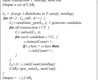
In this paper, we use apriori-like method to discover all CARs. On the mining tasks, firstly the algorithm discovers all the CARs in dataset D. The algorithm for discovering CARs is given in Figure 1.
CARs algorithm consists of the same number of passes as the Apriori. Initially, L
1contains all the 1-RuleItems that satisfy the minimum support threshold. This is done by scanning the whole dataset one time. During pass k, the algorithm discovers the set of frequent k-RuleItems and then generates CAR
kthat satisfies the minimum confidence. The algorithm terminates when L
kis empty.
Input transaction T, minSup, minConf Output a set of CAR
kL
1= {Large 1-RuleItems in T satisfy, minSup}
for (k=2 ; L
k-1≠Ø ; k++) {
C
k=candidate_gen(L
k-1); // generate candidate for all transaction t ∈ T {
C
t=subset(C
k, t);
for each candidate c ∈ C
t{ c.itemsetCount++;
if c.class = t.class then c.ruleCount++;
} }
L
k={c | c.ruleCount≥minSup}
CAR
k=gen_rule(L
k, minConf);
}
Output = ∪
kCAR
kFigure 1. Outline of algorithm for discovering CARs.
4. BUILDING CLASSIFICATION USING CARS After CARs are discovered, the resulting set of CARs can still be huge and contain many uninformative redundant CARs.
All the CARs nedd to be ranked and only the most highly ranked CARs will be inserted into classifier. The rank can be measured by either the cohesion measure itself or by some other criteria. After being sorted in decreasing rank order, the CARs are pruned using database coverage pruning.
4.1 CAR Cohesion Measure and CARs Ranking CAR Cohesion measure is used for CARs ranking. CARs ranking is needed to select the best CARs in case of overlapping CARs. The proposed CAR Cohesion measure is adapted from the cohesion measure as defined below.
Definition 4.1: For a CAR (item
1,…,item
n)→C of length n, CAR Cohesion is a ranking measure defined as
n 1 n
n 1 n
1
) C ( Count ) item ( Count ) item ( Count
) C , item ,..., item ( Count )
C , item ,..., item (
Cohesion =
where Count(item
1,…,item
n, C) is a number of transactions where the itemsets and class occur together, Count(item
i), i=1,…,n, is a number of transactions containing item
i, and
Count(C) is a count of transactions classified to class C in a training set.
Cohesion measure is higher if the item
1,…,item
nand C co- occur more frequently in the together and are less frequently encountered separately.
CARs ranking guarantees that only the highest rank CARs will be selected into the classifier. All CARs are ranked according to the following criteria.
Definition 4.2: CARs Ranking, given two rules CAR
iand CAR
j, CAR
i>CAR
j(or CAR
iis ranked higher than CAR
j) if
(1) Cohesion(CAR
i)>Cohesion(CAR
j) or
(2) Cohesion(CAR
i)=Cohesion(CAR
j) but Frequency(CAR
i)>Frequency(CAR
j) or
(3) Cohesion(CAR
i)=Cohesion(CAR
j) and Frequency(CAR
i)=Frequency(CAR
j) but
support(CAR
i)>Support(CAR
j)
A rule CAR
1: X → C is said a general rule w.r.t. rule CAR
2: X' → C', if only if X is a subset of X'. First, we need to sort the set of generated CARs for each k-star expression and then given two rules CAR
1and CAR
2, where CAR
1is a general rule w.r.t CAR
2, we prune CAR
2if CAR
1also has higher rank than CAR
2. The rationale behind the prune is the following: if rule CAR
icovers a case d then sub-rule of CAR
ialso covers it, and sub- rule will always be selected since it has higher rank.
4.2 Database Coverage Pruning
After the CARs are ranked and sorted in decreasing rank order, the highest ranked CARs are selected into classifier, while the others are pruned using database coverage pruning.
We use coverage pruning like that in [Li 2001]. Database coverage pruning ensures that every CAR selected into the classifier classifies correctly at least one data case and that each training data case is covered by several CARs of the highest possible rank. The Figure 2 shows the process of database coverage pruning.
Input a training data set D, a set of CARs R, coverage threshold ε .
Output a set of CARs SR used by classifier, a default rule DR.
(1) DR={the majority class in D, C
m};
(2) for each case d
i⊆ D cover count dcover
i=0;
(3) SR= Ø ;
(4) for ( training data set D= Ø or R= Ø ) do { (5) for each CAR
i⊆ R do {
(6) find a set D
cover⊆ D of cases covered by CAR
iand D
cover. ∈ CAR
i(7) if at least one d ⊆ D
coveris correctly classified by CAR
ithen {
(8) SR = SR∪CAR
i;
(9) for each case d
j⊆ D
coverand do { (10) dcover
j++;
(11) if dcover
j= ε then (12) delete d
jfrom D;
(13) } (14) } (15) } (16) }
Figure 2. Database coverage pruning algorithm.
3 First for each case in D, set its cover-count to 0. If CAR can
correctly classify at least one case then select CAR and increase the dcover of those cases matching CAR by 1. A case is removed if its dcover passes coverage threshold. A default rule is also selected. It has an empty rule and predicts a class label, which is a majority class among the case left in D or if none is left is the majority class in the original database. After a set of rules is selected for classifier, we classify new cases. We discover the rules matching case in the selected one and classify class labels of the discovered rules. If all the rules matching the new case have same class label, the new case is assigned to that label.
5. EXPERIMENTAL RESULTS
In this section, we evaluate our experiments of the proposed anomaly detection model on the dataset from the DARPA’98 Intrusion Detection Evaluation. The DARPA program that was prepared and managed by MIT Lincoln Labs[DARPA 1998]
has provided the dataset. A standard set of data to be audited, which includes a wide variety of intrusions simulated in a military network environment, was provided.
The DARPA training data consists of seven weeks of network-based attacks. Attacks are labeled in the training data.
To preprocessing the training data, we use connections as the basic granule, obtaining the connection from the raw packet data of the audit trail. We preprocess the packet data in the training data files in the following schema :
R=(Src_IP, Src_Port, Dest_IP, Dest_Port, Class) where Src_IP and Src_Port denote source address and port number respectively, while Dest_IP and Dest_Port, represent the destination address and Port number. The attribute Class is class labels that are two categories: attack and normal. Figure 3 depicts the preprocessing results TCP-dump data from raw packet data of audit trail.
0 –0 – laodmodule0 – portsweep
… 192.168.001.001 192.168.001.001 194.007.248.153 172.016.113.050 172.016.113.050
… 192.168.001.005 172.016.112.020 172.016.113.084 197.218.177.069 205.160.208.190
… 8053 2523 1… 110653 205041026 1234… domain/uhttp
telnetsmtp tcpmux
… 00:00:01 00:00:02 00:00:01 00:00:26 00:00:01
… 08:00:01 08:00:01 08:00:01 11:46:39 11:49:39
… 07/03/1998 07/03/1998 08/03/1998 07/03/1998 07/03/1998
… 12 83833 9966…
Attack Score/Name IP addressDest IP addressSrc
DestPort PortSrc Service Duration Start Start Time
# Date
preprocessing preprocessing
normal normal normal attack attack
… 8053 2523
…1 192.168.001.001 192.168.001.001 194.007.248.153 172.016.113.050 172.016.113.050
… 110653 205041026
1234… 192.168.001.005 172.016.112.020 172.016.113.084 197.218.177.069 205.160.208.190
…
Intrusion Dest_port Dest_ip Src_port Src_ip
normal normal normal attack attack
… 8053 2523
…1 192.168.001.001 192.168.001.001 194.007.248.153 172.016.113.050 172.016.113.050
… 110653 205041026
1234… 192.168.001.005 172.016.112.020 172.016.113.084 197.218.177.069 205.160.208.190
…
Intrusion Dest_port Dest_ip Src_port Src_ip
0 –0 – laodmodule0 – portsweep
… 192.168.001.001 192.168.001.001 194.007.248.153 172.016.113.050 172.016.113.050
… 192.168.001.005 172.016.112.020 172.016.113.084 197.218.177.069 205.160.208.190
… 8053 2523 1… 110653 205041026 1234… domain/uhttp
telnetsmtp tcpmux
… 00:00:01 00:00:02 00:00:01 00:00:26 00:00:01
… 08:00:01 08:00:01 08:00:01 11:46:39 11:49:39
… 07/03/1998 07/03/1998 08/03/1998 07/03/1998 07/03/1998
… 12 83833 9966…
Attack Score/Name IP addressDest IP addressSrc
DestPort PortSrc Service Duration Start Start Time
# Date
preprocessing preprocessing
normal normal normal attack attack
… 8053 2523
…1 192.168.001.001 192.168.001.001 194.007.248.153 172.016.113.050 172.016.113.050
… 110653 205041026
1234… 192.168.001.005 172.016.112.020 172.016.113.084 197.218.177.069 205.160.208.190
…
Intrusion Dest_port Dest_ip Src_port Src_ip
normal normal normal attack attack
… 8053 2523
…1 192.168.001.001 192.168.001.001 194.007.248.153 172.016.113.050 172.016.113.050
… 110653 205041026
1234… 192.168.001.005 172.016.112.020 172.016.113.084 197.218.177.069 205.160.208.190
…
Intrusion Dest_port Dest_ip Src_port Src_ip
normal normal normal attack attack
… 8053 2523
…1 192.168.001.001 192.168.001.001 194.007.248.153 172.016.113.050 172.016.113.050
… 110653 205041026
1234… 192.168.001.005 172.016.112.020 172.016.113.084 197.218.177.069 205.160.208.190
…
Intrusion Dest_port Dest_ip Src_port Src_ip
normal normal normal attack attack
… 8053 2523
…1 192.168.001.001 192.168.001.001 194.007.248.153 172.016.113.050 172.016.113.050
… 110653 205041026
1234… 192.168.001.005 172.016.112.020 172.016.113.084 197.218.177.069 205.160.208.190
…
Intrusion Dest_port Dest_ip Src_port Src_ip
Figure 3. Preprocessing of the training dataset.
Our experiment focused on DoS and Probe attacks since there appear to be no sequential patterns that are frequent in records of R2L and U2R
We have two important thresholds for the classifier performance(minSup, Database coverage). These thresholds control the number of frequent CARs selected for constructing classifier in our experiments. We carried out experiments using different thresholds over random samples of training dataset, 10% of total size. Figure 4 show classifier average classification error according to support and database coverage respectively where minConf=0.6.
36 38 40 42 44 46 48 50
0.001 0.002 0.004 0.005 0.01
minimum support
avg. error ra
dbcover=2 dbcover=4 dbcover=5 dbcover=6 dbcover=8 dbcover=10
Figure 4. Classifier accuracy on training data.
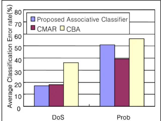
Based on Figure 4, for our algorithm, the minimum support is set to 0.004 and the database coverage is set to 5. The minimum confidence and minimum frequency are set to 0.5 and 0.6 respectively. We compare accuracy of our algorithm, CMAR [Li 2001] and CBA[Liu 1998]. The result is shown on Figure 5.
0 10 20 30 40 50 60 70 80
DoS Prob
Average Classification Error rate(%)
CMAR CBA
Proposed Associative Classifier
CMAR CBA
0 10 20 30 40 50 60 70 80
DoS Prob
Average Classification Error rate(%)
CMAR CBA
Proposed Associative Classifier