IEG 환경지질연구정보센터

(1)

1. Introduction

Change detection techniques using multi-temporal satellite images have been continuously developed and applied. They can be divided into two fields: the detection of detailed change properties, and binary

change detection, which focuses on extracting only the area of change.

Binary change detection is a method for separating the changed area from the unchanged area in multi- temporal satellite images. The most important steps in the process are the application of various change

Application of Multiple Threshold Values for Accuracy Improvement of an Automated Binary Change

Detection Model

Byeong-Hyeok Yu*^†and Kwang-Hoon Chi*^,**

*Department of Geoinformatic Engineering, University of Science & Technology

**Geoscience Information Department, Korea Institute of Geoscience & Mineral Resources

Abstract :Multi-temporal satellite imagery can be changed into a transform image that emphasizes the changed area only through the application of various change detection techniques. From the transform image, an automated change detection model calculates the optimal threshold value for classifying the changed and unchanged areas. However, the model can cause undesirable results when the histogram of the transform image is unbalanced. This is because the model uses a single threshold value in which the sign is either positive or negative and its value is constant (e.g. -1, 1), regardless of the imbalance between changed pixels. This paper proposes an advanced method that can improve accuracy by applying separate threshold values according to the increased or decreased range of the changed pixels. It applies multiple threshold values based on the cumulative producer’s and user’s accuracies in the automated binary change detection model, and the analyst can automatically extract more accurate optimal threshold values. Multi- temporal IKONOS satellite imagery for the Daejeon area was used to test the proposed method. A total of 16 transformation results were applied to the two study sites, and optimal threshold values were determined using accuracy assessment curves. The experiment showed that the accuracy of most transform images is improved by applying multiple threshold values. The proposed method is expected to be used in various study fields, such as detection of illegal urban building, detection of the damaged area in a disaster, etc.

Key Words :

Automated binary change detection model; multiple threshold values; cumulative producer’s and user’s accuracies, IKONOS.

Received June 12, 2009; Revised June 29, 2009; Accepted June 29, 2009.

†Corresponding Author: Byeong-Hyeok Yu ([email protected])

(2)

detection techniques to emphasize the changed area, and application of an appropriate threshold method for separating the changed area. Much related research has been implemented and reported (Lu et al., 2004).

Many studies have focused on methods for determining the optimal threshold values for separating the changed from the unchanged area. In general, methods for detecting optimal threshold values are of two types: one is based on the analyst ’ s adjustment by trial and error; the other is based on the standard deviation or an accuracy assessment curve (Morisette and Khorram, 2000). In general, an accuracy assessment curve has been preferred because it can quantitatively compare the corresponding accuracy for each threshold value (Lunetta et al., 2002; Lu et al., 2005). However, these optimal threshold values have limits because the method uses only a few values and does not reflect the directionality of change of the pixels.

Therefore, this paper proposes an advanced method that can implement more accurate binary change detection by combining the advantages of both methods. It defines each optimal threshold value for the lowest and highest portions in the whole range, and also improves accuracy by complementing the omitted parts of the changed area.

2. Determination of Optimum Threshold Values

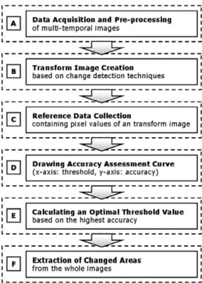
1) Single optimal threshold based on an automated binary change detection model The study range of this research is limited to the binary change detection model using an accuracy assessment curve, which was introduced by Morisette and Khorram (2000). In general, these models follow the processing steps shown in Fig. 1. (A) First, for the

purpose of binary change detection, multi-temporal satellite images need to be acquired and basic pre- processing implemented, such as geometric correction, radiometric normalization, etc. (B) The different change detection techniques for emphasizing only the changed area in the multi- temporal images were introduced by Lu et al. (2004) in detail. A new transform image can be created by applying an appropriate change detection technique to the pre-processed multi-temporal satellite images.

(C) Reference data is created from the transform image, and the pixel values of the transform image are collected according to their location. (D) To display an accuracy assessment curve, an analyst separates the changed from the unchanged pixels, based on a threshold value defined from all the pixels of the transform image, and creates an error matrix. A detailed description of the error matrix can be found

Fig. 1. Processing steps of a general binary change detection model.

(3)

in Morisette and Khorram (2000). From the error matrix, different classification accuracies (e.g. the Kappa coefficient, overall accuracy, user’s accuracy, and producer’s accuracy) can be calculated, and the individual accuracy for each threshold value can be displayed as an accuracy assessment curve. (E) In the accuracy assessment curve, an optimal threshold value is calculated based on the highest accuracy. (F) Finally, the changed area is separated from the whole image using this value.

The basic binary change detection model determines threshold values according to an analyst’s subjective decision, so trial-and-error procedures are required. Lunetta et al. (2002) also used standard deviation values as threshold values.

In recent research, Im et al. (2007) developed a method which can continuously increase threshold values according to the constant interval on a wide range of threshold values, and can display a more precise accuracy assessment curve. This method also presented a module that automatically dispenses with the burdensome steps required for binary change detection, and is defined as an automated binary change detection model.

In particular, the model disposes of step (D) in Fig. 1.

Here, T means the threshold and V

_start

, V

_end

, and V

_step

mean the start value, end value, and step value defined by the analyst, respectively, while V

_pix

means the pixel value of each reference point. The abbreviations used in the error matrix are shown in Fig. 2.

for T = start V

_start

, end V

_end

, step V

_step

if abs(V

_pix

) ≥ T then (1) the class value = ‘change’

or

the class value = ‘no change’

end if

makes the error matrix . . . (2) clsref = {(Cg

_cls

× Cg

ref

) + (NCg

_cls

×

NCg

_ref

)}

Kappa = {N

_total

× (Cg

clsref

+ NCg

_clsref

)) - clsref} / {(N

_total

)2 - clsref} (3) next

First, the threshold value is increased stepwise as the step value between the start and end values. Each pixel value is classified into either a changed class, in which the value is more than the threshold value, or an unchanged class, and an error matrix is formed from these values. The Kappa accuracy is calculated using Eq. (3), and the process is repeated for the whole threshold range. The threshold value having the highest Kappa accuracy is defined as the optimal threshold value, and it becomes the base for extracting the changed area.

In Eq. (1), the directionality of the changed pixel value is not considered because the pixel value of the transform image is converted into an absolute value.

In other words, the threshold values for positive and negative ranges are equal and opposite in sign. For example, if the threshold is 1, the actual threshold values will be -1 and 1. This is based on the fact that the histogram of the transform image generally shows the normal (Gaussian) distribution. The proposed method has the advantage of being able to extract a more accurate optimal threshold value than the previous model. However, some changed areas may be omitted if the histogram of the transform image is not a normal distribution, because the directionality of pixel values in the changed area is not considered.

Fig. 2. Error matrix abbreviations of a binary change detection model.

(4)

2) Accuracy assessment curves based on cumulative producer’s and user’s accuracies (PUAs)

The simplest method for considering the directionality of the changed area is to calculate optimal threshold values separately in the lowest and highest ranges of the transformation histogram distribution.

However, the Kappa coefficient can result in a relatively complex calculation when using the lowest and highest ranges, because it combines all cells of the error matrix for its calculation. Also, if ten threshold values in each range are calculated, one hundred calculations, including the consideration of all cells, will be required. Therefore, the Kappa coefficient is limited by a time delay in repeated accuracy assessment.

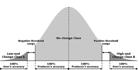
An accuracy assessment curve based on the cumulative producer’s and user’s accuracies (PUAs) as proposed by Cakir et al. (2006), shows results very similar in accuracy to the Kappa accuracy assessment, and has the advantage of a simpler algorithm for calculation. It is based on the fact that each optimal threshold value at the lowest and highest ranges is determined by a peak point having the highest cumulative producer’s and user’s accuracy (Fig. 3). This is expressed in Eq. (4).

PUAs = (Cg

_ref

/ N

_total

) + (Cg

_cls

/ N

_total

) (4) Cakir et al. (2006) used the multiple threshold values of the lowest and highest ranges, but this has limitations for calculating more accurate optimal threshold values, because it used manual threshold values with wide steps.

3. Proposed Method

The proposed method combines the advantages of the two models presented above. That is, it applies multiple threshold values based on PUAs in a repetitive optimal threshold calibration of an automated binary change detection model. Therefore, Eq. (3) is replaced with Eq. (4), and the proposed method for considering the directionality of the transform image is defined below. Here, S

_h

, S

_l

, and S

_t

mean the sample(s) of the high-end range, the sample(s) of the low-end range, and the total sample(s), respectively.

for T = start V

_start

, end V

_end

, step V

_step

select S

_h

from S

_t

(5)

where V

_pix

≥ 0

Fig. 3. Possible multiple threshold range for the changed areas in the histogram distribution of a transform image (Cakir et al, 2006).

(5)

if V

_pix

≥ T then (6) the class value = ‘change’

or

the class value = ‘no change’

end if

PUAs = (Cg

_ref

/ N

_total

) +

(Cg

_cls

/ N

_total

) (7)

repeat, in cases where:

V

_pix

≤ 0 and S

l

In this way, the proposed method repeatedly calculates the classification accuracy in the lowest and highest ranges, so that more accurate optimal thresholds can be produced. In other words, the problem of the single optimal threshold in the automated binary change detection model is solved

by applying the low-end and high-end thresholds differently. This research implements this advanced algorithm into the new module available in ArcGIS 9.x, because it requires an automated repetitive calculation. For the implementation, the ArcObjects Library and Visual Basic for Application (VBA) programming languages were used.

4. Experiment

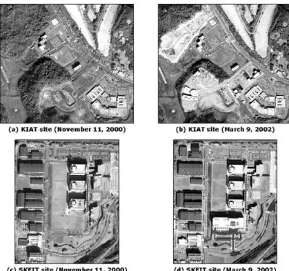
1) Study area and remote sensing data Two institutional sites in Daejeon were selected for this experiment. The first was the Korean Institute of Aerospace Technology (KIAT) site, in which a portion of a forest was removed for a building extension, and the second was the SK Energy

Fig. 4. Panchromatic bands of the multi-temporal IKONOS satellite images obtained from the study area. KIAT means the Korea Institute of Aerospace Technology, and SKEIT also means the SK Energy Institute of Technology, respectively. (a) and (c) show the status before change, and (b) and (d) show the status after change.

(6)

Institute of Technology (SKEIT) site, in which there was new building construction, a parking lot extension, etc. (Fig. 4).

Multi-temporal IKONOS high-resolution satellite imagery was used, and the data acquired was for November 11, 2000 and March 9, 2002, respectively, with a difference of 16.79˚ in the tilt angle (Table 1).

Therefore, change detection results may inevitably include shadows or the sides of tall buildings.

2) Pre-processing

IKONOS imagery acquired 4 m low-resolution multispectral images and 1 m high-resolution panchromatic images respectively, so the first pre- processing involved pan sharpening based on a 1 m spatial resolution. The Gram-Schmidt image fusion method (Aiazzi et al., 2006) was applied, and four pan-sharpened multispectral images and one panchromatic image were used in this study. Also, 10 pseudo-invariant features (PIF) were collected from invariant bare lands and buildings, and the radiometric normalization based on time 1 was implemented.

3) Reference data

Reference data was collected from the whole area by the random sampling method. When collecting pixel values for the equal position of the transform images, the most appropriate transformations can be selected according to a statistical accuracy comparison. In this experiment, 500 points were selected as reference data.

4) Transformations

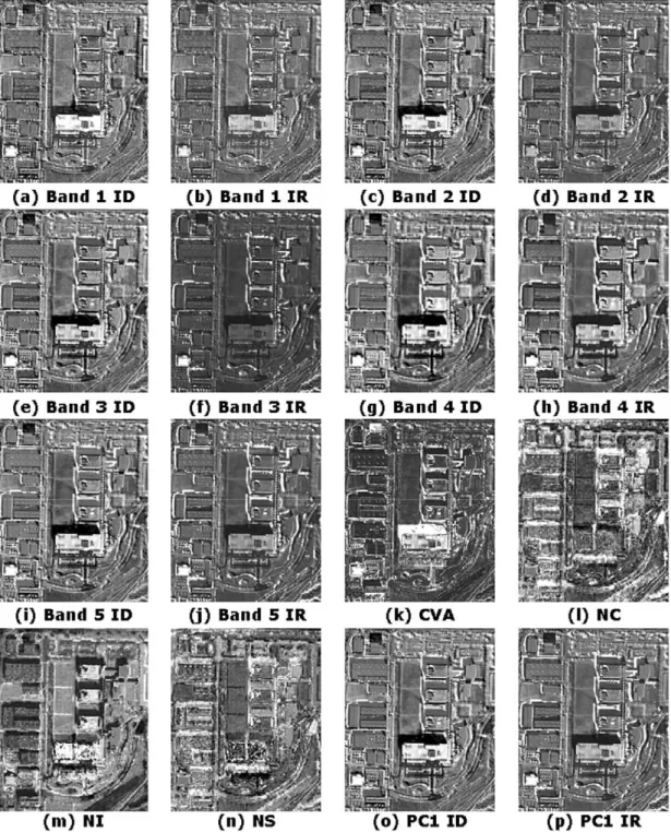
A total of 16 transform images were used for this experiment. Firstly, the application of image differencing (ID) and image ratioing (IR) methods created 10 transform images from the fused multispectral bands and the original panchromatic band. Change vector analysis (CVA) was applied, and neighborhood correlation (NC), neighborhood slope (NS), and neighborhood intercept (NI) transform images were acquired according to the neighborhood correlation image (NCI) method. The NCI method calculates the Pearson’s product moment correlation coefficient from multi-temporal satellite images, and was introduced by Im and Jensen (2005); Im (2006). The principal component analysis (PCA) method was also applied, and the converted PC1 ID and IR results were used.

5. Results and Discussion

In total, 16 transformation results were produced, as in Fig. 5-1 and Fig. 5-2. Fig. 6 shows clearly distinguished transform images, and the classification accuracy actually reflects the degree of change detected. Of course, some methods can only be distinguished clearly by visual analysis, however, such visual analysis is mainly determined by the subjective interpretation of the analyst. Therefore, the transform images were compared to each other based on the classification accuracy of the optimal threshold value.

The proposed method in this research replaces the

Table 1. Remote sensing data characteristics for the two study sites

Study area Sensor Acquisition dateAcquisition time (GMT)Tilt angle Sun azimuth Sun Elevation

Daejeon IKONOS November 11, 2000 2:18 70.57 163.61 34.66

March 09, 2002 2:28 87.36 153.51 45.79

Study area Sensor Acquisition date Acquisition time (GMT) Tilt angle Sun azimuth Sun Elevation

(7)

calculation method for the classification accuracy based on an automated binary change detection model. Therefore, the degree of improvement was assessed by comparing the results of applying a single threshold to those of applying multiple thresholds.

1) Accuracy assessment results of applying a single threshold value

For the two study sites, the results of the optimal threshold and the Kappa accuracy for applying a single threshold are shown in Table 2. For the KIAT site, bands 1, 2, 3, the panchromatic band, and the PC1 ID showed 0.861, 0.874, 0.886, 0.819, and 0.888 Kappa accuracy, respectively, which is relatively

Fig. 5-1. Results transformed from the multi-temporal satellite images in the KIAT site. ID means an image differencing, IR means

an image ratioing, CVA means a change vector analysis, NC means a neighborhood correlation, Ni means a neighborhood intercept, NS means a neighborhood slope, and PC means a principal component, respectively.

(8)

Fig. 5-2. Results transformed from the multi-temporal satellite images in the SKEIT site. ID means an image differencing, IR means an image ratioing, CVA means a change vector analysis, NC means a neighborhood correlation, NI means a neighborhood intercept, NS means a neighborhood slope, and PC means a principal component, respectively.

(9)

high. The CVA showed the highest accuracy, with a value of 0.904. But NC and NS showed low accuracy (0.206 and 0.168, respectively) which indicates that these were inappropriate transformation methods for the study area. The SKEIT site showed a lower classification accuracy than the KIAT site, but the panchromatic band, PC1 ID, and CVA showed high accuracy (0.805, 0.819, and 0.807, respectively).

However, as with the KIAT site, NC and NS could not determine the changed area.

2) Accuracy assessment results applying multiple threshold values

The results of the optimal threshold and the classification accuracy of applying multiple threshold values are shown in Table 3. CVA and NC were eliminated from the multiple thresholds because they

have no directional properties. The multiple threshold values are actually calculated from the PUAs, but the Kappa accuracy was additionally calculated for comparison with the single threshold value.

For the KIAT site, bands 1, 2, 3, and the panchromatic band ID showed high accuracy at 0.880, 0.894, 0.867, and 0.839, respectively. Band 1 IR also showed high accuracy (0.821), and the PC1 ID showed the highest at 0.919. For the SKEIT site, the PC1 ID showed the best accuracy at 0.896, similar to the KIAT site, and bands 2, 3, and the panchromatic band ID showed high accuracy at 0.866, 0.872, and 0.867, respectively.

3) Result comparison between single and multiple threshold values

Fig. 7 shows the accuracy assessment curves

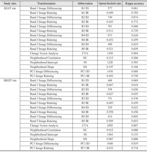
Fig. 6. Transform images and Kappa accuracies in the two study sites. (a)-(c) were acquired from the KIAT site, and the others were acquired from the SKEIT site. (a), (d) means the lowest values, (b), (e) means the moderate values, and (c), (f) means the highest values.

(10)

Table 2. Optimal single threshold values and Kappa accuracies calculated from an automated binary change detection model Study sites Transformation Abbreviation Optimal threshold value Kappa accuracy

KIAT site Band 1 Image Differencing B1 ID 577 0.861

Band 1 Image Ratioing B1 IR 0.499 0.785

Band 2 Image Differencing B2 ID 749 0.874

Change Vector Analysis CVA 1458 0.904

Neighborhood Correlation NC 0.212 0.206

Neighborhood Intercept NI 1220 0.565

Neighborhood Slope NS 0.197 0.168

PC1 Image Differencing PC1 ID 1438 0.888

PC1 Image Ratioing PC1 IR 0.493 0.758

SKEIT site Band 1 Image Differencing B1 ID 468 0.669

Change Vector Analysis CVA 1095 0.807

Neighborhood Correlation NC 0.912 0.000

Neighborhood Intercept NI 1564 0.153

Neighborhood Slope NS 0.987 0.000

PC1 Image Differencing PC1 ID 1048 0.819

PC1 Image Ratioing PC1 IR 0.632 0.718

Study sites Transformation Abbreviation Optimal threshold value Kappa accuracy

(11)

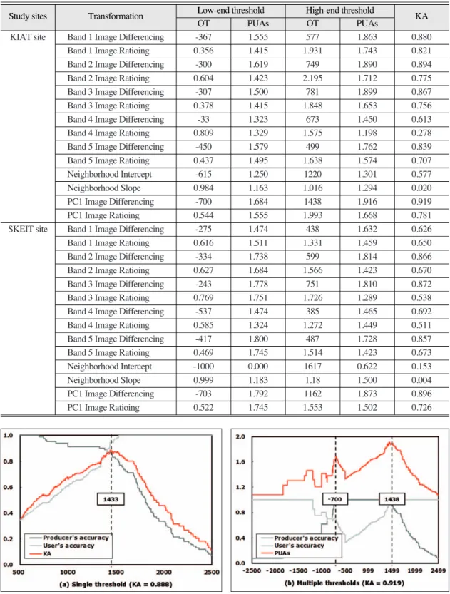
Table 3. Optimal multiple threshold values and Kappa accuracies calculated from the cumulative producer’s and user’s accuracies (PUAs). OT means the optimal threshold value and KA means the Kappa accuracy

Study sites Transformation Low-end thresholdHigh-end thresholdKA

OT PUAs OT PUAs

KIAT site Band 1 Image Differencing -367 1.555 577 1.863 0.880

Band 1 Image Ratioing 0.356 1.415 1.931 1.743 0.821

Band 2 Image Differencing -300 1.619 749 1.890 0.894

Neighborhood Intercept -615 1.250 1220 1.301 0.577

Neighborhood Slope 0.984 1.163 1.016 1.294 0.020

PC1 Image Differencing -700 1.684 1438 1.916 0.919

PC1 Image Ratioing 0.544 1.555 1.993 1.668 0.781

SKEIT site Band 1 Image Differencing -275 1.474 438 1.632 0.626

Neighborhood Intercept -1000 0.000 1617 0.622 0.153

Neighborhood Slope 0.999 1.183 1.18 1.500 0.004

PC1 Image Differencing -703 1.792 1162 1.873 0.896

PC1 Image Ratioing 0.522 1.745 1.553 1.502 0.726

Study sites Transformation Low-end threshold High-end threshold

OT PUAs OT PUAs KA

Fig. 7. Results comparison applying the single and multiple threshold values for the PC1 image differencing image in the KIAT site.

When the multiple threshold values are applied to an automated binary change detection model, the changed areas of the negative range (from -1433 to -701) are additionally detected.

(12)

displayed when the single and multiple threshold values were applied respectively against the PC1 ID image for the KIAT site. In (a), an optimal threshold value was defined by Kappa accuracy, with an approximate 0.888 classification accuracy. In (b), optimal threshold values were calculated using PUAs, and it was determined that PUAs showed the highest accuracy. The Kappa accuracy was calculated from multiple threshold values at 0.919. This means that the multiple threshold values additionally detected the changed area that was previously omitted (from -1433 to -701).

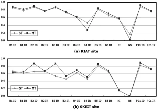
For the second study site, the comparison of Kappa accuracies for single and multiple threshold values are shown in Fig. 8 and Table 4. First, for the KIAT site (a), the accuracy of the transform images was improved for all but 4 images, for the SKEIT site (b),

the accuracy of all but one transform image was improved. In the case of site (a), especially, the accuracy of PC1 ID was increased from 0.888 to 0.919, and was higher than the CVA (0.904), the highest value when a single threshold was used. Also, for site (b), the accuracies of bands 2 and 3 ID were greatly increased, by 0.210 and 0.335, respectively.

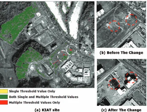
Fig. 9-1 and Fig. 9-2 show the binary change mask results when applying single and multiple threshold values in the automated binary change detection model. For the PC1 ID, which had the highest accuracy, it was confirmed that the changed area, which was not detected in the case of the single threshold, was now detected for both the KIAT and SKEIT sites.

Fig. 8. Kappa accuracies comparison of the single threshold (ST) and the multiple threshold (MT) values in the two study areas. In KIAT site, most Kappa accuracies were increased except B3 ID, B4 ID, B4 IR, and NS. In SKEIT site, all Kappa accuracies were increased except only B1 ID.

(13)

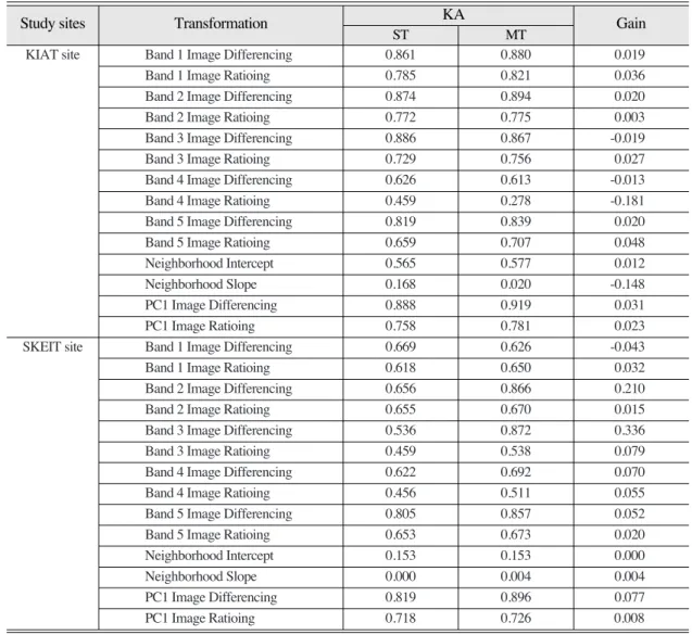
Table 4. Kappa accuracies and gain values according to the single and multiple threshold values in the two study sites. KA means Kappa accuracy, ST means the single threshold value, and MT means the multiple threshold values

Study sites Transformation KA Gain

ST MT

KIAT site Band 1 Image Differencing 0.861 0.880 0.019

Band 1 Image Ratioing 0.785 0.821 0.036

Band 2 Image Differencing 0.874 0.894 0.020

Band 3 Image Differencing 0.886 0.867 -0.019

Band 4 Image Differencing 0.626 0.613 -0.013

Band 4 Image Ratioing 0.459 0.278 -0.181

Neighborhood Intercept 0.565 0.577 0.012

Neighborhood Slope 0.168 0.020 -0.148

PC1 Image Differencing 0.888 0.919 0.031

PC1 Image Ratioing 0.758 0.781 0.023

SKEIT site Band 1 Image Differencing 0.669 0.626 -0.043

Neighborhood Intercept 0.153 0.153 0.000

Neighborhood Slope 0.000 0.004 0.004

PC1 Image Differencing 0.819 0.896 0.077

PC1 Image Ratioing 0.718 0.726 0.008

Study sites Transformation KA

ST MT Gain

(14)

Fig. 9-1. Binary change masking result for the PC1 image differencing image in the KIAT site. It shows that the use of multiple threshold values additionally detect portions of the changed area.

Fig. 9-2. Binary change masking result for the PC1 image differencing image in the SKEIT site. It shows that the use of multiple threshold values additionally detect portions of the changed area.

(15)

6. Conclusion

This paper proposed an advanced method that can achieve more accurate change detection by altering the determination step for optimal threshold values in the automated binary change detection model. The proposed method replaces a single threshold with multiple thresholds. In addition, omitted changed areas could also be detected. It is particularly beneficial when the histogram of the transform image shows, or is likely to show, non-Gaussian distribution.

In the experimental results, it was proved that the proposed method could improve the classification accuracy of most change detection techniques. The proposed method is expected to be used in various study fields such as illegal urban building detection, damaged area detection after disasters such as floods or landslides, etc.

References

Aiazzi, B., Baronti, S., Selva, M., and Alparone, L., 2006. Enhanced Gram-Schmidt spectral sharpening based on multivariate regression of MS and Pan data, Proc. of Geoscience and Remote Sensing Symposium 2006, 3789- 3792.

Cakir, H. I., Khorram, S., and Nelson, S. A. C., 2006.

Correspondence analysis for detecting land cover change, Remote Sensing of Environment, 102: 306-317.

Im, J. and Jensen, J. R., 2005. A change detection model based on neighborhood correlation image analysis and decision tree classification, Remote Sensing of Environment, 99: 326-340.

Im, J., 2006. Neighborhood correlation image analysis for change detection using different spatial resolution imagery, Korean Journal of Remote Sensing, 22(5): 337-350.

Im, J., Rhee, J., Jensen, J. R., and Hodgson, M. E., 2007. An automated binary change detection model using a calibration approach, Remote Sensing of Environment, 106: 89-105.

Lu, D. Mausel, P., Brondizio E., and Moran, E., 2004.

Change detection techniques, International Journal of Remote Sensing, 25(12): 2365- 2407.

Lu, D., Mausel, P., Batistella, M., and Moran, E., 2005.

Land-cover binary change detection methods for use in the moist tropical region of the Amazon: a comparative study, International Journal of Remote Sensing, 26(1): 101-114.

Lunetta, R. S., Ediriwickrema, J., Johnson, D. M., Lyon, J. G., and McKerrow A., 2002. Impacts of vegetation dynamics on the identification of land-cover change in a biologically complex community in North Carolina, USA, Remote Sensing of Environment, 82: 258-270.