1. Introduction
For a sustainable development of a watershed, building accurate inventories and monitoring of wetlands at risk are very important. Recently inventory maps for natural resources have been constructed using remote sensing techniques, but classification accuracy of
inland wetlands was doubtful, because Spectral similarities among wetlands, agricultural fields and forest can create difficulties in classifying satellite images (Houhoulis and Mitchener 2000).
Wetlands are lands with a mixture of water, herbaceous or woody vegetation and wet or saturated soils and LSMA technique is one of the most often used
Linear Spectral Mixture Analysis of Landsat Imagery for Wetland Land-Cover Classification
in Paldang Reservoir and Vicinity
Sang-Wook Kim* and Chong-Hwa Park**
Land Research Institute, Korea Land Corporation*
Graduate School of Environmental Studies, Seoul National University**
Abstract : Wetlands are lands with a mixture of water, herbaceous or woody vegetation and wet soil.
And linear spectral mixture analysis (LSMA) is one of the most often used methods in handling the spectral mixture problem. This study aims to test LSMA is an enhanced routine for classification of wetland land-covers in Paldang reservoir and vicinity (Paldang Reservoir) using Landsat TM and ETM+
imagery. In the LSMA process, reference endmembers were driven from scatter-plots of Landsat bands 3, 4 and 5, and a series of endmember models were developed based on green vegetation (GV), soil and water endmembers which are the main indicators of wetlands. To consider phenological characteristics of Paldang Reservoir, a soil endmember was subdivided into bright and dark soil endmembers in spring and a green vegetation (GV) endmember was subdivided into GV tree and GV herbaceous endmembers in fall. We found that LSMA fractions improved the classification accuracy of the wetland land-cover. Four endmember models provided better GV and soil discrimination and the root mean squared (RMS) errors were 0.011 and 0.0039, in spring and fall respectively. Phenologically, a fall image is more appropriate to classify wetland land-cover than spring’s. The classification result using 4 endmember fractions of a fall image reached 85.2 and 74.2 percent of the producer’s and user’s accuracy respectively. This study shows that this routine will be an useful tool for identifying and monitoring the status of wetlands in Paldang Reservoir.
Key Words :
LSMA, Endmember Identification, Wetland Land-cover.Received 12 April 2004; Accepted 21 May 2004.
methods in handling the spectral mixture problem.
However, wetland studies using LSMA technique mostly focused on the vegetation factor (Blaricom et al., 1996; Williams et al., 1999) and there is little research to take into account soil and water factors for identification and classification of wetlands.
This study aims to test fraction images developed from LSMA can improve classification accuracy of wetland land-cover, and to achieve an appropriate processing routine of LSMA. It is possible to obtain better results if the mixed pixels of wetlands are decomposed into different proportions of vegetation, soil and water components, which are the three main indicators of wetlands. Moreover, this study was conducted to determine the optimum time of a year to classify wetlands using two season’s remotely sensed data.
Although LSMA has been recognized as an effective method in handling spectral mixture problems, some uncertainties are still not understood. This paper contributes to answer some uncertainties of LSMA. For example, how many and what kind of endmembers were suitable for wetland classification?, how to select endmembers manually? and which season is more appropriate to detect wetland land-cover between spring and fall?
2. Study Area and Data Used
1) Study Area
Paldang reservoir and catchment protection area and vicinity areas of four km buffers from the main river channels of Hangang, Namhangang, Bukhangang and Kyungancheon River (Paldang Reservoir), were designated as the focal area for this study. The dominant flora in Paldang area are cattail (Typha angustata), reed (Phragmites communis), water chestnut (Trapa
japonica) community, and so on. The possibility of accurate classification of wetland land-cover may be increased by comparing seasonal characteristics of spring and fall seasons. Phenologically in May, cattails grow to maturity but rice is transplanted to paddy fields in Paldang Reservoir. In September, rice and cattails are in maturity but the understory background material of paddy fields is wet soil, while the background of wetlands is saturated soil (Kim and Park, 2003).
2) Field Survey
Basically wetland distributions were investigated from digital maps from the Ministry of Environment.
Among 49 wetlands in Paldang Reservoir, locations and types (seasonal or perennial) of 31 wetlands were detected based on ‘Land-Cover Maps’ (1/25,000) and
‘Land Environment Maps’ (1/25,000). And 18 wetlands omitted from those maps were detected from the field survey, which were registered with GPS (Trimble Pathfinder) device to allow integration with spatial data in GIS and image processing systems. The appearance of obligate or facultative wetland vegetation was the main indicator for wetland identification in the field survey. To overcome the inaccessibility to some of wetlands and mapping exact location of them, wetland locations were checked directly by loading the maps onto PDA connected to the GPS receiver. Spatial data were processed and integrated as GIS layers using ENVI 3.6 and ArcView v3.2
3. Methodology
1) Endmember Identification
For endmember identification, laboratories at U.S.
Geological Survey, Jet Propulsion Laboratory and
John’s Hopkins University have been supplying several
spectral libraries, and many studies have adopted
spectral libraries for endmember identifications (Roberts et al., 1998; Winter 1999; Drake et al., 1999; Sabine et al., 2002; Kim, 2003). In this study endmembers were selected from pure features in the imagery, because spectral libraries, which offer spectral values of minerals, soils and vegetations of the U.S environment are rare for Korean natural ecosystems, and utilizing field spectrometers are not readily available to researchers.
One approach for choosing endmembers from imagery is selecting representative and homogeneous pixels from satellite imagery through visualizing spectral scatter-plots of image band combinations. When each endmember is selected from the scatter-plot, the pixel locations are illustrated in the imagery. For this interactive and geometric endmember selection, comprehensive understanding about the site and empirical portion about imagery characteristics is necessary.
Ordinarily, endmember selection is followed by spectral dimension reduction. To reduce the dimension of the data, Principal Component Analysis (PCA) and Minimum Noise Fraction (MNF) (Boardman et al., 1995) algorithm have been applied (Tu et al., 2001; Lee and Lee, 2003). However, this study did not employ dimension reduction algorithms of PCA or MNF. PCA puts almost 90% of the variances on the first two or three components and minimizes the influence of band to band correlation. Those dimension reduction methods were ordinarily used for hyperspectral images (DiPietro, 2002; Kim, 2003), and scatter-plots between newly created components have difficulties to find the three pointiest pixels (i.e. near the vertices) as endmembers.
From the scattergram of red and near-infrared bands, the spectra of mature paddy field or forest located near the pointiest pixels, But the radiance values of mature wetlands are generally located in inside the simplex (convex hull) due to the background effect of ordinary hydrologic and soil conditions in wetlands. And it has
difficulties of direct determination of the wetland endmember from the simplex. And, decomposition or spectral unmixing of the main wetland components into pieces is necessary.
2) Endmember Models
Numbers of endmembers can be various through the phenological changes of land-cover characteristics (Adams et al., 1995; van Wagtendonk and Root, 2000;
Lu et al., 2002). In Paldang Reservoir, by mid-May in spring, the land-cover of paddy fields is not vegetation but wet and moist soil. Therefore, a soil endmember can be specified into bright and dark soil endmembers. In fall, however, vegetation types of forest, paddy and grass are in mature by mid-September. So the GV endmember can be subdivided into GV tree (GVt) and GV herbaceous (GVh) endmembers in Paldang Reservoir. Endmember models for two seasons which are as follows;
a) Spring Image
- 3-endmember model (GV, Soil, Water)
- 4-endmember model(GV, Bright Soil, Dark Soil, Water)
- 5-endmember model(GVt, GVh, Bright Soil, Dark Soil,Water)
b) Fall Image
- 3-endmember model (GV, Soil, Water) - 4-endmember model(GVt, GVh, Soil, Water) - 5-endmember model(GVt, GVh, Bright Soil, Dark
Soil,Water)
To determine endmembers in Paldang Reservoir,
scatter-plots of bands 3, 4 and 5 were mainly utilized
(Fig. 1). Red band (Band 3) and near infrared band(NIR)
(Band 4) have very distinctive three vertices, which
make it easy to determine endmembers from imagery,
and endmembers from these three vertices shows exact
characteristics of three components of wetlands, such as
GV, soil and water. Contrary to other endmember
pixels, the dark soil (e.g. moist soil) pixels are located
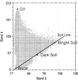
not at a vertex of the scatter-plot but in the middle of the soil line. So, next to the investigation of pure dark soil pixels in images, (e.g. moist soil of paddy fields and barren land near golf links under construction) from site survey and in the two images, the dark soil endmember was selected through the spectral scatter-plot along the soil line (Fig. 1).
To subdivide GV endmember into GVt(GV tree) and GVh(GV herbaceous) for the four and five-endmember models, the scatter-plot of Band 4 and Band 5 was also used. The GVt endmember was identified at the top of the scatter-plot and the GVh endmember was identified at the right vertex of the band 4 and band 5 scatter-plot (Fig. 2). When selecting the endmembers, trial and error needs be taken to identify endmembers precisely. An average of 10 to 15 pixels (endmember bundles) of theses vertices was calculated.
The important thing is to validate whether each land- cover determined in the scatter-plot, is pure to be an endmember or not. Therefore, after the endmember determination from the imagery, purity of illustrated pixels were investigated through field surveys and on- screen certification using a SPOT 5 high spatial resolution image of Paldang Reservoir.
3) Classification of Wetland Land-cover using LSMA Fractions
To evaluate LSMA is an effective processing routine or not, and which season is more appropriate to detect wetland land-cover, four different processing methods
Fig. 1. Identification of GV, Bright Soil, Dark Soil and Waterendmembers in the spring image.
Fig. 2. (a) Identification of GVt, Soil, and Water in the scatter-plots of the bands 3 and 4 in the fall image. (b) GVh, Soil and Water endmembers in the scatter-plots of the bands 4 and 5.
(a) (b)
213
161
109
57
5
Band 4
Band 3
17 46 76 106 136
Band 4
Band 3 137
102
68
34
0
0 54 108 162 217
238
178
119
59
0
Band 5
Band 4
0 40 72 103 135
were tested and their classification results using a maximum likelihood classifier (MLC) were compared.
In supervised classification method, training set data for five land-cover classes of forest, agriculture (e.g.
paddy and dry field and grass), waterbody, bare land (including urban areas, roads and bare soil) and wetland, were collected and defined according to the land-cover characteristics of Paldang Reservoir and vicinity. Every training set of five land-cover classes were extracted from GPS points, general knowledge of the field site (e.g. field notes) and SPOT 5 high spatial resolution image. Training set polygons were created on a geo- referenced true-color display of the image by matching features in the images visually around Paldang Reservoir. The following is four different methods to compare the classification accuracy.
1) MRS : MLC using raw 6-band spring TM image 2) MFS : MLC using fraction images on 6-band
Spring TM image
3) MRF : MLC using raw 6-band fall ETM+ image 4) MFF : MLC using fraction images on 6-band fall
ETM+ image
After the land-cover classification using four methods, to evaluate the accuracy of wetland distribution, each wetland class was selected and segmented to vector layers to be overlaid on the GIS dataset of the study site. Through the segmentation procedure, wetland segments of something small below the 40 pixels (2.7ha) were eliminated. Segmented wetlands were converted to polygons for the effective comparison of location. Error matrices were calculated by comparing the relationships between the location points of wetlands (from GPS points and the digital topographic maps) and classified and segmented wetland polygons.
4. Results and Discussions
1) Comparison of Endmember Models
Land-cover types of Paldang Reservoir vary greatly by the phenological cycle. For both the spring and fall imagery, each mean value of RMS error from three, four
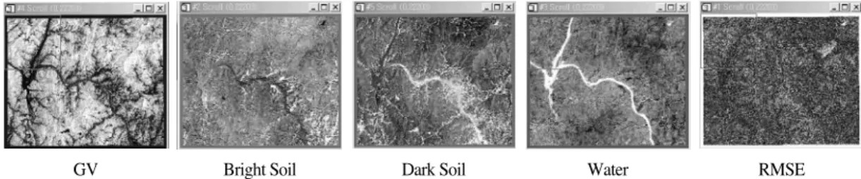
Fig. 3. Fraction images from Spring TM image (May 21, 1999).
GV Bright Soil Dark Soil Water RMSE
Fig. 4. Fraction images from fall ETM+ image (Sept. 23, 2001).
GV tree GV herbaceous Soil Water RMSE
and five endmember model was compared.
In Table 1, the RMS error of five-endmember model has the least RMS error, but the fraction images poorly described the bright soil and dark soil conditions in Paldang Reservoir. The Dark soil fraction image is not consistent with paddy or fields in seeding or transplanting in Paldang Reservoir. The four - endmember unmixing developed high quality fraction images and the normalized Mean RMS value is 0.011, which suggests a generally good fit (less than 0.02, see more Wu and Murray 2002). So in this study, Considering RMS error and visual interpretation of fraction images simultaneously, LSMA result of the four-endmember model of GV, bright soil, dark soil and water were adopted for wetland classification (Table 1).
In case of the fall image (Table 2), the RMS error and fraction images have similar trends with those of spring, and fall ETM+ image might best be represented by the four-endmember model.
2) Fraction Results from LSMA
In the spring image of the four-endmember model, the GV endmember was selected from a forest area
(adjacent to ridgeline covered with Mongolian Oak (Quercus mongolica) community), in the Yongmunsan Mountain in Yangpyong-gun. The dark soil endmember was selected from paddy field area near Namhangang River, and bright soils were selected from bare-land of golf-links under construction and built-up areas of Yangpyong-eup. The water endmember were selected from the deep clear water near Sonaesum Island of Paldang Reservoir.
In case of fall ETM+ image (September 23, ‘01), GV endmember was subdivided into GVt and GVh in order to describe the various vegetation types exactly. The GVt endmember was chosen from a forest area of the south-east side of the valley near Namhangang River.
The GVh endmember was selected from paddy field area near Kangsang-myeon using scatter-plot of band 4 and band 5. The soil endmember was chosen from a construction site in Chonjinam sacred ground. And the pixels of water endmember were selected as same as the spring’s.
In the fraction set, brighter pixels mean higher abundance of the endmember. For Spring TM image (Fig. 3) in the GV fraction map, forests have significan- tly higher values, while paddy fields and built-up areas have very small fraction values. In the dark soil fraction, core areas of paddy fields have relatively higher values than others and in the bright soil fraction, built-up areas have higher values. The last one is the RMS error fraction image and some bright pixels shows the residuals estimated from the unmixing.
In the GVt fraction of the fall scene, forests and wetlands have relatively higher fraction values than those of paddy fields. In the GVh fraction, paddy fields and golf links have higher fraction values and water and forest have lower fraction values (Fig. 4). In the soil fraction, barren lands and built-up areas have the highest values and agricultural lands have higher values than those of wetlands. In September, both aquatic plants and paddy fields are in maturity, but the understory
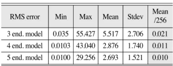
Table 1. RMS error comparison for the selection ofappropriate endmember selection (Spring Image, May 21, 1999).
RMS error Min Max Mean Stdev Mean /256 3 end. model 0.035 55.427 5.517 2.706 0.021 4 end. model 0.0103 43.040 2.876 1.740 0.011 5 end. model 0.0100 29.256 2.693 1.521 0.010 RMS error Min Max Mean Stdev Mean /256
Table 2. RMS error comparison for appropriate endmember selection (Fall Image, Sept. 23, 2001).
RMS error Min Max Mean Stdev Mean /256 3 end. model 0.029 46.231 2.176 1.166 0.0082 4 end. model 0.000 41.853 1.0345 0.834 0.0039 5 end. model 0.001 11.099 0.9589 0.485 0.0036 RMS error Min Max Mean Stdev Mean
/256
background materials of paddy fields are wet soil, while the background of wetlands is saturated soil or water land-cover (Fig. 4).
3) Assessment of Classification Accuracy of Wetland Land-cover
Error matrices are often used to assess identification accuracy by comparing the relationship between ground-truth data (reference data) and classified results (Congalton, 1991). The producer’s accuracy and user’s accuracy were calculated based on error matrices.
Reference data from the exact wetland locations from GPS and ancillary maps were used to quantify the accuracy of wetland distribution.
Table 3 summarizes the identification accuracy using 6 different methods. Wetland location points and classified wetland polygons were compared and error matrices of classification accuracies from four methods were calculated for quantitative comparison (Table 3).
In case of MRS and MFS, producer’s and user’s accuracy are very low. It implies that in spring time, wetland condition being in initial growth and development, make it difficult to identify exact areas of wetland land-covers. And similar phenological cycle from growing to mature of wetlands and forests, makes it difficult to classify wetlands and forests.
Phenologically, the LSMA of fall images produced more accurate classification results. If the primary purpose of the classification is to map the locations of the wetland land-cover, we might note that the producer’s accuracy of fall imagery are quite good, and
this would potentially lead one the conclusion that it is adequate for the purpose of detecting the wetland land- cover. But in case of MRF, the user’s accuracy is lower than those of MFF. In case of MRF, even though 86.2%
of the wetland areas have been correctly identified as
‘wetland’, only 64.8% of the areas were identified as
‘wetland’ within the identification are truly of that category. So, concerning which methods are appropriate to, the MFF is the most appropriate one.
5. Conclusions
This study investigated the use of the LSMA in classification of the wetland land-cover in Paldang Reservoir. Several endmember models and classification methods were compared for their success in determining the spatial extent of the wetlands.
Based on the results, the following conclusions can be achieved :
1. LSMA fractions are more appropriate to classify wetland land-covers than when using raw bands of Landsat imagery. And this routine will be helpful to detect wetlands in regional scale. The MFF result using four endmember fractions of a fall image produced 85.2 and 74.2 percent of the producer’s and user’s accuracy respectively.
2. Phenologically, a fall image is more appropriate to classify the wetland land-cover than that of spring in Paldang Reservoir.
3. Considering phenological characteristics to select endmembers, is crucial for developing high quality fraction images using LSMA. The mean RMS error values of four-endmember models of spring (GV, water, dark soil and bright soil) and fall (GV tree, GV herbaceous, soil and water), were 0.011 and 0.0039 respectively, and those suggest generally good fit (less than 0.02).
As a future study, for the type classification of
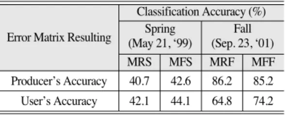
Table 3. Comparison of classification Accuracy from fourdifferent methods.
Error Classification Accuracy (%)
Matrix Spring Fall
Resulting (May 21, ’99) (Sep. 23, ’01)
MRS MFS MRF MFF
Producer’s Accuracy 40.7 42.6 86.2 85.2 User’s Accuracy 42.1 44.1 64.8 74.2 Classification Accuracy (%) Error Matrix Resulting Spring Fall
(May 21, ‘99) (Sep. 23, ‘01)
MRS MFS MRF MFF