저작자표시-비영리-변경금지 2.0 대한민국 이용자는 아래의 조건을 따르는 경우에 한하여 자유롭게
l 이 저작물을 복제, 배포, 전송, 전시, 공연 및 방송할 수 있습니다. 다음과 같은 조건을 따라야 합니다:
l 귀하는, 이 저작물의 재이용이나 배포의 경우, 이 저작물에 적용된 이용허락조건 을 명확하게 나타내어야 합니다.
l 저작권자로부터 별도의 허가를 받으면 이러한 조건들은 적용되지 않습니다.
저작권법에 따른 이용자의 권리는 위의 내용에 의하여 영향을 받지 않습니다. 이것은 이용허락규약(Legal Code)을 이해하기 쉽게 요약한 것입니다.
Disclaimer
저작자표시. 귀하는 원저작자를 표시하여야 합니다.
비영리. 귀하는 이 저작물을 영리 목적으로 이용할 수 없습니다.
변경금지. 귀하는 이 저작물을 개작, 변형 또는 가공할 수 없습니다.
공학석사 학위논문
An Improved SMWI Processing of Substantia Nigra Using
Accurate Phase Combination and Deep Neural Network Based QSM
정확한 위상 합성과 심층 신경망 기반 QSM을 이용한 흑질의 SMWI 영상 개선
2018 년 8 월
서울대학교 대학원
전기정보공학부 전기정보공학전공
조 민 주
An Improved SMWI Processing of Substantia Nigra Using
Accurate Phase Combination and Deep Neural Network Based QSM
지도 교수 이 종 호
이 논문을 공학석사 학위논문으로 제출함 2018 년 8 월
서울대학교 대학원
전기정보공학부 전기정보공학전공 조 민 주
조민주의 공학석사 학위논문을 인준함 2018 년 8 월
위 원 장 심 병 효 (인)
부위원장 이 종 호 (인)
위 원 오 세 홍 (인)
초 록
흑질 구조물인 나이그로좀 1의 자기공명영상은 파킨슨 병의 생체지표로 사용된다. 이 연구에서는 흑질의 자기화율 지도 가중 영상(Susceptibility Map Weighted Image, SMWI)에 사용될 수 있는 두 가지 알고리즘을 제안했다. 우선, 다중 에코 경사 영상(multi-echo gradient echo image) 데이터에서 위상 오프셋을 계산하고 수정하는 방식으로, 다중 에코를 사용하는 다중 채널 위상 조합(Multi-Channel Phase Combination using Multi Echo, MCPC-ME)을 제안하였다. 이 방식의 경우, 모든 에코의 위상 정보를 활용하여 보다 정확한 위상 오프셋 추정이 가능하며, 특히 저(低) 신호 대 잡음 비(SNR) 영역에서 정확도가 높았다. 다음으로 흑질의 자기화율 지도 가중 영상을 도출하는 데 사용되는 자기화율 정량화 영상(Quantitative Susceptibility Map, QSM)의 계산을 위해, 심층 신경 네트워크인 QSMnet을 적용하였다.
이를 이용하여 5.4배 빠른 속도로 나이그로좀 1의 자기화율 정량화 영상을 얻을 수 있었으며, 그로부터 도출된 자기화율 지도 가중 영상은 기존 자기화율 지도 가중 영상과 유사한 영상 대비(image contrast)를 나타내었다.
주요어 : 다중 채널 위상 합성, 자기화율 정량화 영상, 자기화율 지도 가중 영상, 딥 러닝
학 번 : 2016-20979
Content
초 록 ... i
List of Figures ... iii
Chapter 1. Introduction ... 1
1.1 Introduction ... 1
1.1.1 Parkinson’s disease and SMWI image ... 1
Chapter 2. Phase Combination using MCPC-ME ... 5
2.1 Introduction ... 5
2.2 Background ... 5
2.2.1 Preliminary ... 5
2.2.2 MCPC-C ... 6
2.2.3 MCPC-3D... 6
2.2.4 MCPC-ME ... 7
2.3 Methods ... 7
2.3.1 Data acquisition ... 7
2.3.2 Data processing ... 8
2.3.3 Data analysis ... 8
2.4 Results ... 9
2.5 Discussion ... 17
Chapter 3. SMWI with iLSQR-trained QSMnet ... 19
3.1 Introduction ... 19
3.2 Methods ... 21
3.2.1 Data acquisition ... 21
3.2.2 QSMnet ... 22
3.2.3 Data processing ... 24
3.2.4 Data Analysis ... 27
3.3 Results ... 28
3.4 Discussion ... 36
Chapter 4. Conclusion ... 42
References ... 44
Abstract ... 47
List of Figures
Figure 1. Substantia nigra (SN) and nigrosome 1 (N1) region are depicted on a zoomed SMWI image of a healthy subject ... 2 Figure 2.1 Phase image without subtracting phase offsets (at TE=15.42 msec, coil 1, 4, 7, 10) ... 9 Figure 2.2 Phase offsets calculated with MCPC-C (coil 1, 4, 7, 10) ... 10 Figure 2.3 Phase images subtracted by phase offsets calculated with MCPC-C (at TE=15.42 msec, coil 1, 4, 7, 10) ... 10 Figure 2.4 Phase offsets calculated with MCPC-3D (median filtered, coil 1, 4, 7, 10) ... 11 Figure 2.5 Phase images subtracted by phase offsets calculated with MCPC-3D (using median filtered phase offsets, at TE=15.42 msec, coil 1, 4, 7, 10) ... 12 Figure 2.6 Phase offsets calculated with MCPC-3D (median filtered, coil 1, 4, 7, 10) ... 12 Figure 2.7 Phase images subtracted by phase offsets calculated with MCPC-3D (using median filtered phase offsets, at TE=15.42 msec, coil 1, 4, 7, 10) ... 13 Figure 2.8 Representative phase offset map of MCPC-3D and MCPC-ME, without and with median filtering (coil 1) ... 14 Figure 2.9 Combined phase image after subtraction of phase offsets estimated by (a) MCPC-C, (b) MCPC-3D (no filtering), (c) MCPC- ME (no filtering) (d) MCPC-3D (median filtered) and (e) MCPC- ME (median filtered) (at TE=15.42 msec) ...
... 15 Figure 2.10 Q factor map of (a) MCPC-C, (b) MCPC-3D (no filtering), (c) MCPC-ME (no filtering) (d) MCPC-3D (median filtered) and (e) MCPC-ME (median filtered) ... 16 Figure 2.11 Q factor histogram of in-brain voxels ... 17 Figure 2.12 SNR change with Gaussian noise addition ... 18 Figure 3.1 (a) Sagittal view of the image to show the oblique-coronal
orientation of the imaging slab, Multi-Planar Reformatted with respect to the scanner coordinates. (b) Imaging plane view ... 21 Figure 3.2 Summary of the modified QSMnet structure ... 22 Figure 3.3 Summary of the data processing pipeline. ... 25 Figure 3.4 QSM result from iLSQR and QSMnet of a healthy subject from Siemens scanner ... 29 Figure 3.5 QSM results of three test dataset from the two scanners.
... 31 Figure 3.6 SMWI result from iLSQR and QSMnet of a healthy subject from Siemens scanner ... 33 Figure 3.7 SMWI results of three test dataset from the two scanners ... 35
Chapter 1. Introduction
1.1 Introduction
1.1.1 Parkinson’s disease and SMWI image
Parkinson’s disease (PD) is a neurodegenerative disorder which mainly affects motor function [1]. The cause of Parkinson's disease has not yet been fully elucidated. However, many studies reported the decline of motor function in the PD patient can be explained by lack of dopaminergic cells in the brain [1]. Dopaminergic neurons are believed to be involved in the control of voluntary movements and behavioral processes [2]. Substantia nigra pars compacta (SNPC) in the midbrain is formed of dopaminergic neurons. As the use of MR imaging expands in the clinical field, there is an increasing need to establish MR imaging protocols visualizing reduction of dopaminergic cells in PD patients [3-9]. A few studies suggested visualization of the nigrosome 1, a sub-region of substantia nigra (SN), can be an MR imaging biomarker for PD [10-15].
Figure 1. Substantia nigra (SN) and nigrosome 1 (N1) region are depicted on a zoomed SMWI image of a healthy subject. The region confined by the blue line is nigrosome 1 region. The slice orientation is oblique-coronal.
There exists a susceptibility contrast between nigrosome 1 and the other areas in the SN due to the difference in the iron concentration.
Magnetic susceptibility based imaging, such as T2*-weighted imaging, susceptibility weighted imaging (SWI) and Susceptibility map weighted imaging (SMWI), are well-known MR imaging techniques that allow visualization of the changes in dopaminergic neurons in SNPC [10-21]. In healthy controls, this imaging technique generates higher magnetic susceptibility induced tissue contrast between nigrosome 1 and the surrounding SN. Cotrarily, the susceptibility- induced tissue contrast between the two regions is significantly reduced in PD patients [15-17].
Researchers have sought to improve the tissue contrast of utilizing
ultra-high field (UHF) MR [15-17]. In studies using UHF MR, the nigrosome 1 was clearly delineated with conventional T2* weighted imaging technique. However, the UHF system is not widely used for clinical applications so far. In the lower field strength (≤ 3T), because of lower susceptibility induced tissue contrast and SNR visualization of the SNPC using conventional T2* weighted imaging technique has been limited [10-14]. SMWI has been proposed to visualize SNPC at lower field strength [18, 19]. In order to improve the susceptibility induced tissue contrast and signal-to-noise ratio (SNR) without consuming additional scan time, root sum squared multi-echo magnitude image from multi-echo gradient echo (GRE) sequence was utilized in SMWI. In addition, the tissue contrast is enhanced by the use of a quantitative susceptibility mapping (QSM) mask. The QSM mask includes the information of the different susceptibilities of nigrosome 1 and the other regions of the SN. As a result, by using SMWI technique, one can clearly identify nigrosome 1 region at lower field strength [18, 19].
Our work is aimed to achieve high accuracy and fast generation of SMWI image, by improving some steps of the processing. Especially, the generation of the QSM mask generation is of interest. The detailed procedure of the QSM mask generation includes the combination of multi-channel phase images at each echo phase images, generation of local field map, QSM processing, thresholding and affine mapping [18, 19]. In this work, we suggest methods to improve the accuracy of the combination of multi-echo phase data and the processing speed of QSM generation. For more accurate
estimation of phase offsets in multi-echo GRE data, Multi-Channel Phase Combination using all multiple echoes (MCPC-ME) is presented. The accuracy of MCPC-ME was compared to the other methods. This work is demonstrated in Chapter 2 Phase Combination using MCPC-ME. To gain a higher processing speed of SMWI of nigrosome 1, we utilized QSMnet to conduct QSM using deep neural network, since the QSM reconstruction is the most time-consuming step of SMWI processing. The time consumed for the reconstruction of QSM and the image quality of QSM and SMWI of nigrosome 1 generated by QSMnet were investigated. The utilization of QSMnet in SMWI processing is presented in Chapter 3 SMWI with iLSQR- trained QSMnet.
Chapter 2. Phase Combination using MCPC-ME
2.1 Introduction
When acquired with a phased array coil, calculation of phase offsets need to be done before the combination of multi-channel phase data.
The phase map from each coil is composed of echo-time-dependent field inhomogeneity and chemical shift terms and an echo-time- independent inherent phase offset term. The latter term originates from B1 field inhomogeneity, coil geometry, and different receiver chain delay which varies in each channel and voxel. Hence, to prevent phase distortion from such inconsistencies, the phase offset term needs to be removed before combining phase data from multiple channels. Several methods have been suggested to estimate the phase offsets, such as Multi-Channel Phase Combination using Constant offsets (MCPC-C) [22] and Multi-Channel Phase Combination using measured 3D phase offsets (MCPC-3D) [23]. In this study, a more accurate estimation of phase offsets in multi-echo GRE data, Multi-Channel Phase Combination using all multiple echoes (MCPC-ME) is presented. The accuracy of each method was investigated with multi-echo GRE data. The accuracy was also compared under a low SNR simulation.
2.2 Background
2.2.1 Preliminary
Once phase offsets are calculated, they are subtracted from the
phase image of the corresponding coil. If the phase acquired by n- th coil at position (x, y) and echo time TE is θn, and phase offset is θoffset,n, then corrected phase θcorrected,l becomes:
θcorrected,n(x, y, TE) = θn(x, y, TE) − θoffset,n(x, y)
Note that this paper assumes phase offset is constant in time.
In the case of no noise, the corrected phase θcorrected,n(x, y, TE) should be the same between the coils. In the presence of noise, multi-channel phase data can be combined as follows:
θcombined(x, y, TE) = ∠ ∑ M eiθcorrected,n(x,y,TE) n
2.2.2 MCPC-C
In MCPC-C [22], phase offsets are assumed to be spatially invariant. Hence, phase offsets are estimated as the mean phase of a center ROI. It is known that the actual phase offset varies with the position. This fact leads to the inconsistency between the corrected phases of the coils in voxels which are distant from the center.
2.2.3 MCPC-3D
In MCPC-3D [23], voxel-specific phase offset is estimated. The phase of a voxel can be modeled with the time-dependent term (2πγ∆B0(x, y)TE) and time-independent term (i.e. phase offset;
θoffset,n(x, y)). If the phase at position (x, y) at echo time TE1 and TE2 is θn(x, y, TE1) and θn(x, y, TE1), then,
θn(x, y, TE1) = 2πγ∆𝐵0(𝑥,𝑦)𝑇𝐸1+ θ𝑅𝑋,𝑙(𝑥,𝑦) θn(x, y, TE2) = 2πγ∆𝐵0(𝑥,𝑦)𝑇𝐸2+ θ𝑅𝑋,𝑙(𝑥,𝑦) .
When there is no noise, the phase offset θoffset,n(x, y) is simply calculated as follows.
θ𝑜𝑓𝑓𝑠𝑒𝑡,𝑛(𝑥,𝑦)=TE1 θn(x, y, TE2) − TE2θn(x, y, TE1) TE1− TE2
2.2.4 MCPC-ME
When multi-echo GRE data is acquired, one can use collected echoes to improve estimation of phase offsets. Given m echoes, a model for the phase in a voxel located in (x, y) and in the n-th coil at echo times becomes,
θn(x, y, TE1) = 2πγ∆B0(x, y)TEm + θoffset,n(x, y) θn(x, y, TE2) = 2πγ∆B0(x, y)TEm + θoffset,n(x, y)
…
θn(x, y, TEm) = 2πγ∆B0(x, y)TEm + θoffset,n(x, y) .
To generate an optimal estimation of the phase offset, a weighted least squares error minimization is performed with the weighting factors that are inverse of variations of noise in order to calculate the phase offset as the best linear unbiased estimator. Since the variation of phase noise [24] is proportional to 1/SNR2, SNR2 is chosen as a weighting factor of the least square.
2.3 Methods
2.3.1 Data acquisition
2D multi-echo GRE data were acquired at 3T MRI using a 32 channel phased array head coil. Scan parameters were: repetition time (TR) = 2000 msec, echo time (TE) = 2.7, 5.88, 9.06, 12.24, and 15.42 msec, flip angle (FA) = 82°, resolution = 0.9 × 0.9 × 1.0 mm3, and total acquisition time (TA) = 8:34 minutes.
2.3.2 Data processing
Phase data were combined by MCPC-C, MCPC-3D, and MCPC- ME. First and second echoes were chosen to generate a phase offset in MCPC-3D. In MCPC-3D and MCPC-ME, phase data were temporally unwrapped before the estimation of phase offset. To have generality in calculating phase offsets with MCPC-3D, the first and second echo were always used, because they have the lowest noise level. Also, phase unwrapping was done by voxel-level temporal unwrapping with first and second echo phase data.
After evaluating the phase offsets, the results were filtered using a 5x5 median filter. The input data for the median filter (i.e. local 5x5 matrix) were columnized and phase maps were unwrapped. MCPC- 3D and MCPC-ME without the median filter were also tested.
2.3.3 Data analysis
In order to quantify the quality of the phase coherence of each result, a Q factor (Q factor = |Σ𝑒𝑖𝜃𝑐𝑜𝑟𝑟𝑒𝑐𝑡𝑒𝑑|
Σ|𝑀𝑒𝑖𝜃| ) [25], was calculated for every voxel. Q factor is a measure of how coherent the phase offset
subtracted phases are. Higher Q factor means high coherence of the corrected multi-channel phases. SNR was calculated using the magnitude of the complex combined results:
𝑀𝑐𝑜𝑚𝑝𝑙𝑒𝑥 𝑠𝑢𝑚= |∑ 𝑀𝑒𝑖(𝜃𝑙−𝜃𝑅𝑋,𝑙)
𝑙
| .
2.4 Results
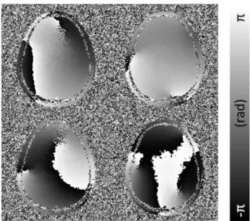
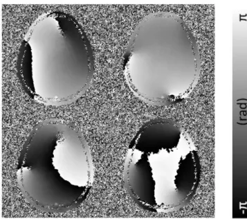
The original phase map, at the fifth echo, is presented in Figure 2.1.
Figure 2.1 Phase image without subtracting phase offsets (at TE=15.42 msec, coil 1, 4, 7, 10)
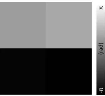
Next, phase offset map and the phase offset corrected map for each method are shown. Figure 2.2 is the phase offset map by MCPC-C, which is constant over each channel, due to the assumption of spatially invariant phase offset.
Figure 2.2 Phase offsets calculated with MCPC-C (coil 1, 4, 7, 10)
Figure 2.3 is the phase offset corrected map by MCPC-C. Corrected phase maps have similar values at the center among the channels, but shows lack of consistency in other areas.
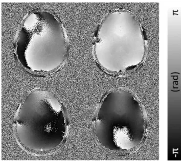
Figure 2.3 Phase images subtracted by phase offsets calculated with MCPC-C (at TE=15.42 msec, coil 1, 4, 7, 10)
Figure 2.4 and 2.5 is phase offset map and corrected phase map by MCPC-3D. The phase offsets are spatially varying and the corrected phase map has good consistency among channels. In Figure 2.5, some in-brain areas that seem very noisy are called as “poles” at that channel, the in-brain regions with low SNR in magnitude image.
Figure 2.4 Phase offsets calculated with MCPC-3D (median filtered, coil 1, 4, 7, 10)
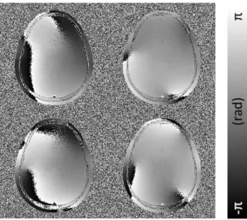
Figure 2.5 Phase images subtracted by phase offsets calculated with MCPC-3D (using median filtered phase offsets, at TE=15.42 msec, coil 1, 4, 7, 10)
Figure 2.6 and 2.7 is phase offset map and corrected phase map by MCPC-ME. MCPC-ME has similar phase offsets with MCPC-3D but with less noise, and it shows better consistency among channels in corrected phase maps.
Figure 2.6 Phase offsets calculated with MCPC-3D (median filtered, coil 1, 4, 7, 10)
Figure 2.7 Phase images subtracted by phase offsets calculated with MCPC-3D (using median filtered phase offsets, at TE=15.42 msec, coil 1, 4, 7, 10)
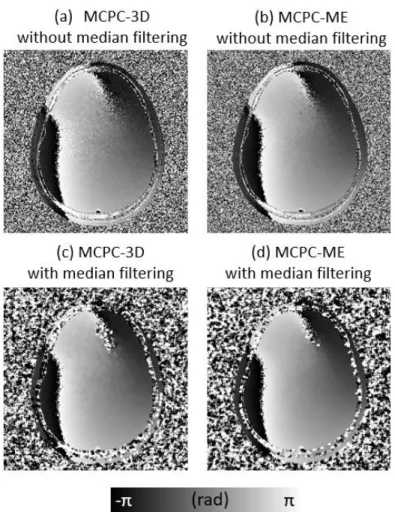
In Figure 2.8, phase offset maps of a representative slice by MCPC- 3D and MCPC-ME, without and with median filtering are compared.
Without median filtering, a map with MCPC-3D is noisier.
Figure 2.8 Representative phase offset map of MCPC-3D and MCPC-ME, without and with median filtering (a) MCPC-3D without median filtering, (b) MCPC-ME without median filtering, (c) MCPC- 3D with median filtering, and (d) MCPC-ME with median filtering (at coil 1)
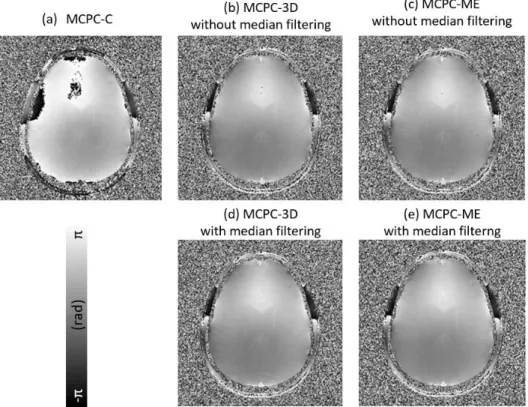
Phase offset subtracted and combined phase maps by MCPC-C, MCPC-3D, and MCPC-ME, both without and with median filtering are compared in Figure 2.9.
Figure 2.9 Combined phase image after subtraction of phase offsets estimated by (a) MCPC-C, (b) MCPC-3D (no filtering), (c)
MCPC-ME (no filtering) (d) MCPC-3D (median filtered) and (e) MCPC-ME (median filtered) (at TE=15.42 msec)
The Q factor map of each method is presented in Figure 2.10.
MCPC-C is less effective in areas away from the center. And while the other methods show relatively low Q factor in the center, median filtered MCPC-ME showed highest Q factor value in the center.
Figure 2.10 Q factor map of (a) MCPC-C, (b) MCPC-3D (no filtering), (c) MCPC-ME (no filtering) (d) MCPC-3D (median filtered) and (e) MCPC-ME (median filtered)
Q factor histograms of in-brain voxels are plotted in Figure 2.11.
The average Q factor for MCPC-C was 0.643 and MCPC-3D and MCPC-ME without filtering were 0.954 and 0.979, respectively.
After median filtering, these values changed to 0.981 and 0.986, respectively. Hence the MCPC-ME shows higher Q values than MCPC-3D although the improvement is relatively small.
Figure 2.11 Q factor histogram of in-brain voxels
2.5 Discussion
MCPC-ME is started from the speculation that it is natural to utilize information from all echoes to increase the accuracy of phase calculation under the circumstance with the noise. To test the effects of the noise level in each method, Gaussian noise at 3 different levels was added to uncombined channel data. To quantitatively measure the effect of noise level on phase offset calculation, SNR of combined magnitude image at second echo was inspected. This result is shown in Figure 2.12. The effect of MCPC-ME becomes larger when the SNR of the image becomes lower. For example, the SNR in MCPC- ME was larger by 56.3% (without the median filter; 19.6% with median filter) than MCPC-3D when the SNR is under 100 (Figure
2.12).
Figure 2.12 SNR change with Gaussian noise addition
The limitation of this work is that phase unwrapping sometimes fails with simple phase unwrapping algorithm provided by MATLAB, especially in later echoes. Failure in phase unwrapping leads to an inaccurate calculation of phase offsets. Utilization of more elaborate phase unwrapping methods will prevent the issue. However, it is likely to fail on unwrapping in frontal areas of the brain, due to their extreme B0 inhomogeneity.
The work is applicable to all kinds of multi-echo multi-channel phase data with linear phase accumulation to improve the accuracy of phase offset calculation, especially when there are not enough SNR.
Chapter 3. SMWI with iLSQR-trained QSMnet
3.1 Introduction
In the SMWI processing, QSM reconstruction for the QSM mask generation is the most time-consuming step. QSM estimates susceptibility source distribution from local field map [26]. Local field map is a phase map induced by the convolution of the susceptibility source and dipole kernel. By duality, Fourier transform of susceptibility can be calculated from Fourier transform of local field map divided by Fourier transform of dipole kernel. However, because Fourier transform of dipole kernel has zeros on the “magic angle” surface (i.e., 54˚ with respect to the main magnetic field), calculation of susceptibility map has an ill-posed problem [26].
Several algorithms have been introduced to solve the problem in the QSM. Calculation of susceptibility through multiple orientation sampling (COSMOS) is a method to overcome the lack of information on zero cone surface by acquiring multiple orientation data with respect to the main magnetic field [27]. Requiring extra scan time, such strategy demands more cost and may provoke patients' inconvenience.
In order to solve the ill-posed problem in the single orientation QSM data, algorithms that iteratively search the solution that satisfies the data consistency between the local field map and the dipole convolution of susceptibility map and the prior knowledge are widely
used [28-30]. For instance, iLSQR exploits the prior knowledge that first order derivatives are not necessarily zero at zero cone surface when iteratively estimating susceptibility map [28, 29]. These sorts of strategies require longer calculation time because of their iterative behavior. Recently, a method named QSMnet which utilizes U-net [31] structure to conduct QSM reconstruction has been proposed [32]. This deep neural network was trained with local field maps and the corresponding COSMOS results. Compared with conventional QSM reconstruction algorithms, QSMnet showed faster reconstruction time and higher consistency among orientations.
In our work, we utilized QSMnet to conduct QSM using deep neural network to gain higher processing speed of SMWI of nigrosome 1.
However, QSMnet is not directly applicable to the QSM reconstruction of the SMWI data due to the difference in the resolution and the orientation. In addition, the data for the imaging of substantia nigra lack of data size along the z-direction, and the orientation of each data is different from one another. Since the data were different from the original QSMnet training set data, the data and QSMnet have to be modified for appropriate training. Therefore, QSMnet layers and training sets are modified according to the data characteristic and the deep neural network are trained. The time consumed for the reconstruction of QSM and the image quality of QSM and SMWI of nigrosome 1 generated by QSMnet were investigated with test set data.
3.2 Methods
3.2.1 Data acquisition
All MR scans were conducted on 3T clinical MR scanners using 32- channels received phased-array head coil. This study was approved by the Institutional Review Board, and all participants provided written informed consent.
Figure 3.1 (a) Sagittal view of the image to show the oblique-coronal orientation of the imaging slab, Multi-Planar Reformatted with respect to the scanner coordinates. (b) Imaging plane view. Both images are root sum squared multi-echo magnitude image of each echo of GRE image.
For train and test of QSMnet, data from two distinct MRI scanners and imaging parameters were used. Out of the total 62 subjects, 44 subjects were scanned with Siemens scanner (3T Skyra). The other 18 subjects were obtained from Philips scanner (3T Achieva).
For both data acquisitions, 3D multi-echo GRE sequence was used.
The data were acquired with a single orientation. Spatial resolution was 0.5 × 0.5 × 1.0 mm3, and field of view was 192 × 192 × 32 mm3. In order to minimize the partial volume effect imaging plane was aligned with ‘oblique-coronal’ line (dotted red line in Figure 3.1 (a)).
The typical acquired image is shown in Figure 3.1 (b).
Specific scan parameters were as follows:
(Siemens 3T Scanner)
TR = 88 ms, TE = 12, 24, 36, 48, 60, 72 ms, FA = 10°, readout bandwidth = 100 Hz/pixel, GRAPPA acceleration factor = 2 and acquisition time (TA) = 7:30.
(Phillips 3T Scanner)
TR = 48 ms, TE = 14, 27, 40 ms, FA = 20°, and readout bandwidth = 100 Hz/pixel, SENSE acceleration factor = 2, and TA = 4:15.
3.2.2 QSMnet
structure is the same as QSMnet [32], but the innermost layers are not included.
To conduct deep learning-based image to image operation, QSMnet [32], which is a modified version of U-net [31] structure with 3D inputs and outputs, was utilized. Detailed network architecture used in our study is illustrated in Figure 3.2. The network was modified to exclude the innermost convolution, deconvolution and feature concatenation layers with 512 channels.
Same loss function which proposed by Yoon et al. was used for QSMnet training [32]. The loss function is represented as follows,
Loss = w1∙ (𝑚𝑜𝑑𝑒𝑙 𝑙𝑜𝑠𝑠) + 𝑤2∙ (𝐿1 𝑙𝑜𝑠𝑠) + 𝑤3∙ (𝑔𝑟𝑎𝑑𝑖𝑒𝑛𝑡 𝑙𝑜𝑠𝑠)
= w1 ‖𝑑 ∗ 𝜒 − 𝑑 ∗ 𝑦‖1+ 𝑤2 ‖𝜒 − 𝑦‖1+ 𝑤3 (‖|∇d ∗χ| − |∇d ∗ y|‖1 + ‖|∇χ| − |∇y|‖1)
w1, w2 and w3: weighting factors, d: dipole kernel, χ: output of QSMnet, y: output label
The loss function was the sum of the model loss, L1 loss and gradient loss multiplied by weighting factors. The model loss is a term that imposes the numerically computed local field map from the QSM results, i.e., it matches dipole convolution of QSMnet outputs and output labels. The L1 loss is a term that matches the QSMnet outputs and the output labels. Gradient loss is a term that matches the edge information of the numerically computed local field maps and the QSM maps. Weighting factors are the contributions of the respective loss functions to the total loss function. The network was
implemented with TensorFlow [33] and trained on an NVIDIA 1080TI GPU. Batch size was 5 and training epochs were set to be 100.
3.2.3 Data processing
To solve inverse problem of the QSM for mask generation, phase images were calculated. Phase data obtained with multi-receive channel head coils were combined by applying MCPC-C to the raw data for the Siemens system [22]. For the Phillips system, the multi- channel combined DICOM data were used.
QMSnet was trained with 3D patches from local field map and the corresponding QSM results. In order to apply QSMnet network, training datasets for SN images were modified and had different features with those of previous work reported by Yoon et al [32].
Because the data was acquired with single orientation COSMOS was not applicable. Therefore, iLSQR results were used as the training label. Since the matrix size in the z-direction is relatively smaller than the other directions, the training patch had size limitation along the z-direction. The images were resampled to enlarge the patch size along the z-direction. In order to solve the problem with incoherent image orientations between the subjects, local field maps with various orientations were retrospectively generated for training.
QSMnet estimates the QSM map from the local field map which appears as a convolution of susceptibility and the dipole kernel. Since the dipole kernel is formed according to the orientation with respect
to the main magnetic field, it is hard to guarantee the convergence of the network if the orientation is not consistent. One of the strategies was to let the network learn the relationship of local field map and QSM with various orientations by providing a sufficient number of the images. This strategy was accomplished by retrospectively generating local field map with various orientations from the acquired data. Also during training, dipole kernel according to the orientation was accounted in loss function. This is expected to help the network to learn dipole deconvolution according to each data’s orientation.
Figure 3.3 Summary of the data processing pipeline.
Detailed explanation about QSMnet is described in section 3.2.2.The data processing pipeline is presented in Figure 3.3. GRE phase data were spatially unwrapped with MRPhaseUnwrap function provided in STI Suite v2.2 [34]. To generate local field map, HARPERELLA [34] and iHARPERELLA [34] were applied to unwrapped phase data from Siemens and Philips scanner,
respectively. QSM images were generated by applying iLSQR algorithm [28] (error tolerance: 0.01, threshold k-space regions:
0.1). Local field map and QSM images were sinc-interpolated along the z-direction with resampling factor = 2. Regions with errors in QSM images were discarded manually. Then the QSM data and the corresponding local field maps at remaining regions from 57 subjects (42 from Siemens and 15 from Philips scanner) were dissected into 48 × 48 × 32 voxel-sized patches for train label and train input respectively. Centers of the patches along the x- and y-directions were 24 voxels apart. Along the z-direction, patches were generated with 2 different ways based on the matrix size. When the matrix size was larger than 32, two patches were generated. While the matrix size was smaller than 32 one patch was generated. To discard the data with inaccurate QSM estimation, Fourier transform of dipole kernel with respect to the orientation of each patch was generated.
Fourier transformed dipole kernel was multiplied by Fourier transform of the iLSQR result. Then the result was inverse Fourier transformed and compared with the original local field map. If the portion of the voxels with error rate under 50% was less than 30%, the corresponding patch was discarded. For data augmentation, dipole kernel corresponding to the rotated orientation along the x-, y-, and z-axis of the actual scanner with ±5°from the original orientation was calculated and the kernel was convoluted to the QSM patches to calculate local field maps. This step included formerly discarded patches because local field map is calculated regardless of the
patches have comparable signal intensity range with the label patches, the intensity of the input patches were multiplied by 3.
3.2.4 Data Analysis
For the evaluation of QSMnet results, five datasets which were not used for the training were used as the test sets. For each subject, 32 or 48 consecutive slices including SN were selected. Then, the selected slices from each subject were put into the trained QSMnet.
The time consumed for QSMnet with TensorFlow [33] using NVIDIA 1080TI GPU was inspected and compared with the time consumed for iLSQR algorithm with the same local field map in MATLAB (R2014b, 64bit) on Ubuntu. The QSM images generated by iLSQR algorithm and QSMnet were compared.
To generate SMWI results, QSMnet outputs and iLSQR labels were made into susceptibility mask (Smask) using the following equation:
S𝑚𝑎𝑠𝑘(χ) = {
0 𝑖𝑓 χ > χ𝑡ℎ χ𝑡ℎ− χ
χ𝑡ℎ 𝑖𝑓 0 < χ < χ𝑡ℎ 1 𝑜𝑡ℎ𝑒𝑟𝑤𝑖𝑠𝑒.
χth is a paramagnetic threshold value and was chosen to be 1, as optimized in the previous study [19].
SMWI is produced by multiplication of root sum squared multi-echo GRE magnitude image and the power of the generated mask.
SMWI = (Smask)m × GREmagnitude
The exponent of the Susceptibility mask (m) was chosen to be 4, also as optimized in the previous study [19]. The SWMI images generated by QSMnet and iLSQR outputs were compared. For
quantitative evaluation, nigrosome 1 and the other regions of substantia nigra of healthy subjects were manually drawn on SMWI images made from iLSQR results. Then, contrat-to-noise ratio (CNR) was calculated as the ratio between the mean of nigrosome 1 area and the mean of the other regions of the substantia nigra in the SMWI images. The CNR was calculated for each healthy subject. The left and right regions were considered separately. The statistical significance of the difference of the CNRs was determined by paired samples t-test.
3.3 Results
Obtained three dimensional multi-echo GRE data were processed according to the data processing pipeline shown in Figure 3.3. The total training time of QSMnet was about 25.5 hours. The processing time for the 24 slices SMWI image was reduced by 48.1 sec (59 sec with iLSQR method; 10.9 sec with QSMnet).
Figure 3.4 QSM result from iLSQR and QSMnet of a healthy subject from Siemens scanner. (a) QSM result from iLSQR, (b) QSM result of the same slice from QSMnet, (c) zoomed QSM result from iLSQR, (d) zoomed QSM result from QSMnet, and (e) intensity plot at a 42- nd cross-sectional line of (c) and (d). The cross-sectional line is indicated as a dotted line on (c) and (d). (f) The difference of the two cross-sectional intensity
Figures 3.4 (a) and (b) show typical QSM result reconstructed with iLSQR and QSMnet. A slice which includes SN and nigrosome 1 was selected for comparing results. Figures 3.4 (c) and (d) are the expanded images of the white box in Figures 3.4 (a) and (b) to show the susceptibility induced tissue contrast between nigrosome 1 and the other regions of substantia nigra more closely. The QSM results from QSMnet showed similar tissue contrast with results from iLSQR.
Signal intensity plots along with the dotted black line in Figures 3.4 (c) and (d) are shown in Figure 3.4(e). When the signal intensities of QSM maps from QSMnet and iLSQR were plotted, all of the signal plots demonstrated a similar shape but different magnitudes. The dynamic range of the signal intensity from QSMnet is smaller than that from iLSQR. Especially, the voxels with negative susceptibility values always had lower values in the iLSQR results than that from QSMnet. The difference of the signal intensities between the two methods are shown in Figure 3.4(f). The mean value of the absolute of the intensity difference between the methods of the region near nigrosome 1 was 0.0152.
Figure 3.5 QSM results of three test dataset from the two scanners.
Subject 1-3: healthy, Siemens scanner, subject 4: healthy, Philips scanner, subject 5: Parkinson’s disease, Philips scanner. The slices are zoomed to view substantia nigra and nigrosome 1. Subject 1 is
the same data in Figure 3.4. From the three different subjects, QSM results from iLSQR (left), QSM results from QSMnet (middle), and the difference maps, which are QSMnet results subtracted by iLSQR results (right) are indicated.
All QSM results from the test dataset are shown in Figure 3.5. In Figure 3.5, subject 1-3 showed a slightly weaker contrast in overall QSMnet results than in iLSQR results, as mentioned in Figure 3.4. In contrast, the subject 4 and 5 showed a stronger contrast in QSMnet results than in iLSQR results.
Figure 3.6 SMWI result from iLSQR and QSMnet of a healthy subject from Siemens scanner. (a) SMWI made from iLSQR, (b) SMWI result of the same slice made from QSMnet, (c) zoomed SMWI result from iLSQR, (d) zoomed SMWI result from QSMnet, and (e) intensity plot at a cross-sectional line of (c) and (d). The cross-sectional line is indicated as a dotted line on (c) and (d). (f) The difference of the two cross-sectional intensity
SMWI images generated by using QSM masks from iLSQR and QSMnet are shown in Figure 3.6. The images and plots were made with the same slice and cross-sectional line as in Figure 3.4.
Throughout the Figures 7(a)-(d), no significant differences appeared on the overall images nor the zoomed images near substantia nigra and nigrosome 1. In Figures 7(e), the plot from SMWI by iLSQR and QSMnet showed good agreement. In Figure 3.6(f), the plot of the cross-sectional intensities from the two methods had little difference while QSMnet had smaller intensity usually. The mean value of the absolute of the cross-sectional intensity difference near the nigrosome 1 region (figure 3.6(f)) is 8.3063.
Figure 3.7 SMWI results of three test dataset from the two scanners.
Subject 1-3: healthy, Siemens scanner, subject 4: healthy, Philips
scanner, subject 5: Parkinson’s disease, Philips scanner. The slices are zoomed to view substantia nigra and nigrosome 1. Subject 1 is the same data in Figure 3.6. From the three different subjects, SMWI results made from iLSQR (left), SMWI results made from QSMnet (middle), and the difference maps, which are absolute of QSMnet results subtracted by iLSQR results multiplied by 5 (right) are indicated.
SMWI images made from the QSM results of Figure 3.5 are presented in Figure 3.7. The difference map was the absolute of the difference multiplied by 5. In Figure 3.7, subject 1-3 showed similar or higher intensities in substantia nigra from QSMnet results than from iLSQR results. In contrast, the subject 4 and 5 showed similar or lower intensities in substantia nigra from QSMnet results than from iLSQR results.
For the images of Figure 3.7, the mean of CNR calculated from each pair of ROIs was 1.4382 for SMWI from iLSQR and 1.4257 for SMWI from QSMnet. The p-value of the difference of the eight pairs of CNR values were 0.7237, i.e., no significant difference was found between the CNRs of the SMWI images from iLSQR and QSMnet.
3.4 Discussion
In this work, we demonstrated the utilization of QSMnet to produce the susceptibility mask used in SMWI of nigrosome 1. The processing time was 5.4 times faster with QSMnet than with iLSQR. The comparison was not done under equal condition since QSMnet was implemented with python and was run on GPU while iLSQR was
implemented with MATLAB and was run on CPU. However, QSMnet has a good capacity of parallelization, which would be considered in the comparison.
The QSM and SMWI images produced by iLSQR and QSMnet were compared. In Figure 3.4 (a) and (b), (b) showed a slightly weak contrast than (a) did. The relationship also appeared in Figure 3.4 (e), where QSMnet intensity was higher than iLSQR for negative intensities and lower than iLSQR for positive. The same relationship was found in subject 1 to 3 in Figure 3.5. In contrast, the subject 4 and 5 in Figure 3.5 showed a reversed relationship: the contrast of the QSMnet images of subject 4 and 5 were stronger than the iLSQR images. The reason for this is, as shown in Figure 3.5, that the QSM contrasts generated by iLSQR algorithm varied with respect to the scanner. QSMnet would have been trained to produce intermediate results for both scanner images.
As in Figure 3.6 and 8, the SMWI results showed less prominent relationship than the QSM results, regardless of the MR scanner. The average value of absolute of difference of a cross-sectional line near nigrosome 1 (see Figure 3.4 (f)) was 10.1% to the highest value of iLSQR in QSM, while it was 8.3% in SMWI. We conjectured that the SMWI showed similar contrast than QSM because of the way the susceptibility mask is generated. First, the susceptibility mask is 0 to 1, so the error is confined to a restricted range. Also, negative QSM values were transformed into 1 in QSM mask domain, regardless of the QSM value. Thus, the errors in the QSM value under 0 could not propagate into the SMWI image.
In this work, the training dataset differs from the previous QSMnet study [32] in some respects. The most critical difference was the slice orientation. QSMnet was originally targeted to conduct dipole deconvolution to the data to a fixed orientation (axial), while the data for substantia nigra SMWI imaging were acquired with their orientation not fixed at a certain angle (oblique-coronal). QSMnet does not explicitly take account of the input image orientation. One possible approach to overcome the orientation inconsistency issue is to reslice the images to have consistent orientations. This approach was not utilized in this study because the FOV along the z-direction could not be enough for the reslicing and the reslicing also requires additional processing time. The other strategy, which we utilized, was to have sufficient amount of data with various orientation in the test set in order to help the network learn the relationship of local field map and QSM with various orientations. The substantia nigra image, fortunately, is acquired in a certain range of orientation. The QSM data was convoluted by dipole kernel with only ±5˚ rotation according to the main magnetic field to produce a local field map for the data augmentation. Such rotation in slice orientation may affect little on the contrast of the local field map. This fact would have contributed to the network being successfully trained with the limited amount of data. The exact effect of the data augmentation to the QSMnet training has to be examined in future studies.
Another challenge in QSMnet training was lack of the data along the z-direction, allowing only small patch size. By the interpolation along
step is still practical for the actual application since the slices are gained with anisotropic resolution in actual application scan (i.e., coarser resolution in the z-direction) to achieve sufficient SNR in the limited scan time. We used the anisotropic patch size of 48 × 48
× 32. Since the volume of the patch was still 28% of that was used in the original QSMnet paper, the innermost layers with 512 channels were deleted from QSMnet structure to decrease the degree of freedom.
Since QSMnet is a deep neural network architecture, it is hard to characterize the exact working mechanism of the layers. Thus, we could not confirm that QSMnet actually conducts the dipole deconvolution. In order to help the network to learn based on the physical model, the convolution of dipole kernel was used in the model loss term [32]. Nonetheless, this cannot guarantee the dipole deconvolution of the network because the loss function is only applied when training. Further validation has to be done before the utilization of QSMnet for SMWI processing.
For training, we used both data from the two distinct scanners with different scan parameters. We supposed that the vendors and scan parameters would have little influence on the training accuracy since the target of the training is the relationship between the local field map and the QSM map, which is independent of the scanner. However, we found slightly different relationships between the QSM maps from QSMnet and iLSQR of the test data from the different datasets.
Therefore, the effect of the scanner and the scan parameter in the training set to the results of the QSMnet should be examined.
In the training set, there were data of patients with Parkinson's disease. Therefore, some data's nigrosome 1 contrasts were affected by the disease. We speculated that the visibility of nigrosome 1 will not affect the QSMnet learning the QSM reconstruction because the relationship between the local field map and QSM remains the same regardless of the disease. However, the consequences should be investigated in the future studies. Brain abnormalities or susceptibility that are not trained by QSMnet (i.e., susceptibility values under -0.2 or over 0.2 ppm) can produce an unexpected artifact in QSM result. The artifacts caused by the data from various types of disease need to be examined.
The QSMnet trained in this work can be applied to the data with a resolution lower or equal to 0.5 × 0.5 × 0.5 mm3. In the case of the lower resolution data, an appropriate interpolation had to be done.
The effect of the interpolation to the result also needs a close investigation. Because of the feature concatenation layers, the number of the slices has to be at least 8. The input data is limited to the data with oblique-coronal orientation.
In conclusion, the replacement of the conventional iterative QSM algorithm with QSMnet can enhance the processing speed of SMWI with similar contrast. Since QSM is the most time-consuming step of SMWI processing, QSMnet can help to achieve a higher processing speed of SMWI. SMWI images made from the QSM mask from QSMnet showed similarity with the original SMWI images. The application of QSMnet will be helpful when processing a massive
reconstruction of SWMI.
Chapter 4. Conclusion
In this work, two algorithms were introduced to improve SMWI imaging of substantia nigra. In Chapter 2, MCPC-ME, which calculates the phase offsets from all echoes were suggested. It provided a more accurate estimation of voxel-wise phase offsets, particularly in low SNR. In Chapter 3, we applied QSMnet, a deep neural network for QSM reconstruction, to produce QSM mask used in SMWI. Since the work showed the similar contrast in SMWI results with 5.4 times faster speed, it can help when a large amount of data is to be processed or may contribute to the development of an on- scanner reconstruction of SWMI. Combination of MCPC-ME and QSMnet is not covered in this work, but both can be applied to the reconstruction of SMWI.
References
1. Ali Samii, J.G.N., Bruce R Ransom, Parkinson's disease. The Lancet, 2004. 363(9423): p. 1783-1793.
2. Chinta, S.J. and J.K. Andersen, Dopaminergic neurons. The international journal of biochemistry & cell biology, 2005. 37(5): p.
942-946.
3. Hutchinson, M. and U. Raff, Structural changes of the substantia nigra in Parkinson's disease as revealed by MR imaging. American journal of neuroradiology, 2000. 21(4): p. 697-701.
4. Hu, M., et al., A comparison of 18F-dopa PET and inversion recovery MRI in the diagnosis of Parkinson’s disease. Neurology, 2001. 56(9):
p. 1195-1200.
5. Martin, W.W., M. Wieler, and M. Gee, Midbrain iron content in early Parkinson disease A potential biomarker of disease status. Neurology, 2008. 70(16 Part 2): p. 1411-1417.
6. Yoshikawa, K., et al., Early pathological changes in the parkinsonian brain demonstrated by diffusion tensor MRI. Journal of Neurology, Neurosurgery & Psychiatry, 2004. 75(3): p. 481-484.
7. Chan, L.-L., et al., Case control study of diffusion tensor imaging in Parkinson’s disease. Journal of Neurology, Neurosurgery &
Psychiatry, 2007. 78(12): p. 1383-1386.
8. Pavese, N. and D.J. Brooks, Imaging neurodegeneration in Parkinson's disease. Biochimica et Biophysica Acta (BBA)-Molecular Basis of Disease, 2009. 1792(7): p. 722-729.
9. Gorell, J., et al., Increased iron‐related MRI contrast in the substantia nigra in Parkinson's disease. Neurology, 1995. 45(6): p. 1138-1143.
10. Noh, Y., et al., Nigrosome 1 detection at 3T MRI for the diagnosis of early-stage idiopathic Parkinson disease: assessment of diagnostic accuracy and agreement on imaging asymmetry and clinical laterality.
American Journal of Neuroradiology, 2015. 36(11): p. 2010-2016.
11. Schwarz, S.T., et al., The ‘Swallow Tail’Appearance of the Healthy Nigrosome–A New Accurate Test of Parkinson's Disease: A Case- Control and Retrospective Cross-Sectional MRI Study at 3T. PLoS One, 2014. 9(4): p. e93814.
12. Reiter, E., et al., Dorsolateral nigral hyperintensity on 3.0 T susceptibility‐weighted imaging in neurodegenerative Parkinsonism.
Movement Disorders, 2015. 30(8): p. 1068-1076.
13. Sung, Y.H., et al., Drug-induced Parkinsonism versus idiopathic Parkinson disease: utility of nigrosome 1 with 3-T imaging. Radiology, 2015. 279(3): p. 849-858.
14. Cosottini, M., et al., Comparison of 3T and 7T susceptibility-weighted angiography of the substantia nigra in diagnosing Parkinson disease.
American Journal of Neuroradiology, 2015. 36(3): p. 461-466.
15. Cosottini, M., et al., MR imaging of the substantia nigra at 7 T enables diagnosis of Parkinson disease. Radiology, 2014. 271(3): p. 831-838.
16. Kwon, D.H., et al., Seven‐tesla magnetic resonance images of the substantia nigra in Parkinson disease. Annals of neurology, 2012.
71(2): p. 267-277.
17. Blazejewska, A.I., et al., Visualization of nigrosome 1 and its loss in PD Pathoanatomical correlation and in vivo 7 T MRI. Neurology, 2013.
81(6): p. 534-540.
18. Gho, S.M., et al., Susceptibility map‐weighted imaging (SMWI) for neuroimaging. Magnetic resonance in medicine, 2014. 72(2): p. 337- 346.
19. Nam, Y., et al., Imaging of nigrosome 1 in substantia nigra at 3T using multiecho susceptibility map‐weighted imaging (SMWI). Journal of Magnetic Resonance Imaging, 2017. 46(2): p. 528-536.
20. Haacke, E.M., et al., Susceptibility weighted imaging (SWI). Magnetic resonance in medicine, 2004. 52(3): p. 612-618.
21. Zhang, J., et al., Characterizing iron deposition in Parkinson's disease using susceptibility-weighted imaging: an in vivo MR study. Brain research, 2010. 1330: p. 124-130.
22. Hammond, K.E., et al., Development of a robust method for generating 7.0 T multichannel phase images of the brain with application to normal volunteers and patients with neurological diseases.
Neuroimage, 2008. 39(4): p. 1682-1692.
23. Robinson, S., et al., Combining phase images from multi‐channel RF coils using 3D phase offset maps derived from a dual‐echo scan.
Magnetic resonance in medicine, 2011. 65(6): p. 1638-1648.
24. Gudbjartsson, H. and S. Patz, The Rician distribution of noisy MRI data.
Magnetic resonance in medicine, 1995. 34(6): p. 910-914.
25. Robinson, S.D., et al., Combining phase images from array coils using a short echo time reference scan (COMPOSER). Magnetic resonance in medicine, 2017. 77(1): p. 318-327.
26. Wang, Y. and T. Liu, Quantitative susceptibility mapping (QSM):
decoding MRI data for a tissue magnetic biomarker. Magnetic resonance in medicine, 2015. 73(1): p. 82-101.
27. Liu, T., et al., Calculation of susceptibility through multiple orientation sampling (COSMOS): a method for conditioning the inverse problem from measured magnetic field map to susceptibility source image in MRI. Magnetic Resonance in Medicine, 2009. 61(1): p. 196-204.
28. Li, W., et al., A method for estimating and removing streaking artifacts in quantitative susceptibility mapping. Neuroimage, 2015. 108: p. 111- 122.
29. Li, W., B. Wu, and C. Liu, Quantitative susceptibility mapping of human brain reflects spatial variation in tissue composition. Neuroimage, 2011. 55(4): p. 1645-1656.
30. Liu, T., et al., Morphology enabled dipole inversion (MEDI) from a single‐angle acquisition: comparison with COSMOS in human brain imaging. Magnetic resonance in medicine, 2011. 66(3): p. 777-783.
31. Ronneberger, O., P. Fischer, and T. Brox. U-net: Convolutional networks for biomedical image segmentation. in International Conference on Medical image computing and computer-assisted intervention. 2015. Springer.
32. Yoon, J., et al., Quantitative susceptibility mapping using deep neural network: QSMnet. NeuroImage, 2018.
33. Rampasek, L. and A. Goldenberg, Tensorflow: Biology’s gateway to deep learning? Cell systems, 2016. 2(1): p. 12-14.
34. Li, W., et al., Integrated Laplacian‐based phase unwrapping and background phase removal for quantitative susceptibility mapping.
NMR in Biomedicine, 2014. 27(2): p. 219-227.
Abstract
An Improved SMWI Processing of Substantia Nigra Using
Accurate Phase Combination and Deep Neural Network Based QSM
Minju Jo Dept. of Electrical and Computer Engineering The Graduate School Seoul National University
Visibility of nigrosome 1, a subregion of substantia nigra is used as an MR imaging biomarker of Parkinson’s disease. In this work, we introduced two algorithms for SMWI imaging of substantia nigra. First, we suggested Multi-Channel Phase Combination using Multi-Echo (MCPC-ME), a strategy to calculate and correct phase offsets in multi-echo GRE data. MCPC-ME provided a more accurate estimation of voxel-wise phase offsets particularly in low SNR regions by utilizing phase information from all echoes. Second, we applied QSMnet, a deep neural network for QSM reconstruction, to produce QSM image used in SMWI processing. QSM of nigrosome 1 was reconstructed to have comparable SMWI contrast with 5.4 times faster reconstruction speed compared to the conventional QSM reconstruction algorithm.
Keywords : Multi-channel Phase Combine, QSM, SMWI, Deep neural network
Student Number : 2016-20979