저작자표시-비영리-변경금지 2.0 대한민국 이용자는 ... - s-space

저작자표시-비영리-변경금지 2.0 대한민국 이용자는 아래의 조건을 따르는 경우에 한하여 자유롭게

l 이 저작물을 복제, 배포, 전송, 전시, 공연 및 방송할 수 있습니다. 다음과 같은 조건을 따라야 합니다:

l 귀하는, 이 저작물의 재이용이나 배포의 경우, 이 저작물에 적용된 이용허락조건 을 명확하게 나타내어야 합니다.

l 저작권자로부터 별도의 허가를 받으면 이러한 조건들은 적용되지 않습니다.

저작권법에 따른 이용자의 권리는 위의 내용에 의하여 영향을 받지 않습니다. 이것은 이용허락규약(Legal Code)을 이해하기 쉽게 요약한 것입니다.

Disclaimer

저작자표시. 귀하는 원저작자를 표시하여야 합니다.

비영리. 귀하는 이 저작물을 영리 목적으로 이용할 수 없습니다.

변경금지. 귀하는 이 저작물을 개작, 변형 또는 가공할 수 없습니다.

Master’s Thesis of Engineering

Keypoint-based Deep Learning Approach for Building Footprint

Extraction Using Very High Resolution Satellite and Aerial

Images

고해상도 위성영상 및 항공영상에서의 건물경계추출을 위한 특징점 기반의 딥러닝 접근

February 2021

Department of

Civil and Environmental Engineering Seoul National University

Doyoung Jeong

Keypoint-based Deep Learning Approach for Building Footprint

Extraction Using Very High Resolution Satellite and Aerial

Images

Advisor Yongil Kim

Submitting a master’s thesis of Science December 2020

Department of

Civil and Environmental Engineering Seoul National University

Doyoung Jeong

Confirming the master’s thesis written by Doyoung Jeong

January 2021

Chair (Seal)

Vice Chair (Seal)

Examiner (Seal)

i

Abstract

Building footprint extraction is an active topic in the domain of remote sensing, since buildings are a fundamental unit of urban areas. Deep convolutional neural networks successfully perform footprint extraction from optical satellite images. However, the semantic segmentation approach produces coarse results, such as blurred and rounded boundaries in the output, which are caused by the use of convolutional layers with large receptive fields and pooling layers.

Recently, a series of studies has been conducted to directly create polygon representations that describe geometric objects of vector structures through an end-to-end learnable approach. The objective of this thesis is to derive visually improved building objects by directly extracting vertices of independent buildings, which is accomplished by combining instance segmentation and keypoint detection. The target keypoints in building extraction are points of interest based on the local image gradient direction, that is, the vertices of a building polygon. The proposed framework follows a two-stage, top-down approach that that is divided into object detection and keypoint estimation. Keypoints between instances are distinguished by merging the rough segmentation masks and local features of regions of interest. A building polygon is created by grouping the predicted keypoints through a simple geometric method.

In this study, public datasets, namely SpaceNet 2 and Open Cities AI Challenge dataset were used for building footprint extraction. SpaceNet 2 contains satellite images of WorldView-3, which are not orthoimages, while Open Cities AI consists of orthorectified aerial images where annotations match roof outlines and building footprints.

The most widely used semantic segmentation model (EfficientNet–U-Net) and an instance segmentation network (Mask R-CNN) were implemented here to validate the performance of the proposed framework. The framework

ii

was evaluated with three metrics, namely, F1 score, intersection over union (IoU), and structural similarity index measure (SSIM).

The results demonstrated that the proposed framework exhibited better segmentation performance compared with Mask R-CNN in terms of both qualitative and quantitative results under keypoint estimation. However, compared with the state-of-the-art EfficientNet–U-Net, which is based on semantic segmentation, the proposed network performed poorly. This is because the performance of the framework largely depends on the performance of the object detector. Nevertheless, the proposed framework, limited to the detected object in the preceding network, directly predicts the corner points of the building polygon to derive vectorized objects only from the output of the end-to-end learnable network. The proposed framework trains the geometric coordinates of the polygon’s keypoints and demonstrates the potential to directly generate vectorized representations of segmented objects in the satellite images.

Keyword : Building Footprint Extraction, Keypoint Detection, Instance Segmentation, Deep Learning, Satellite image

Student Number : 2019-20867

iii

Table of Contents

Chapter 1. Introduction ... 1

1.1. Background and Motivation ... 1

1.2. Research Objectives ... 5

1.2.1. Workflow ... 5

1.2.2. Contribution ... 7

1.3. Organization of Thesis ... 8

Chapter 2. Related Works ... 9

2.1 Deep Learning for Object Detection and Segmentation . 9

2.1.2. Instance Segmentation ... 10

2.2 Building Footprint Extraction ... 11

2.2.1. Semantic Segmentation ... 13

2.2.2. Instance Segmentation ... 17

2.3 Keypoints Detection ... 19

2.4 Open Datasets for Building Footprint Extraction .... 21

Chapter 3. Backbone Network ... 25

3.1. Feature Extraction ... 27

3.2. Localization ... 28

3.2.1. Region Proposal Network ... 28

3.2.2. Localization Layer ... 29

3.2.3. RoI Allign ... 30

3.3. Loss Function ... 31

iv

Chapter 4. Proposed Framework ... 33

4.1. Instance Segmentation ... 34

4.2. Keypoint Estimation ... 36

4.3. Grouping Keypoints ... 39

Chapter 5. Experimental Design ... 40

5.1. Data Characteristics ... 40

5.2. Implementation Detail ... 43

5.2.1. Data Pre-Processing ... 43

5.2.2. Network Implementations and Configuration ... 44

5.2.3. Training and Testing Details ... 45

5.3.Metrics for Quantitative Analysis ... 46

Chapter 6. Results and Discussion ... 48

6.1. Building Extraction Accuracy ... 48

6.2. Impact of Detectors ... 50

6.3. Keypoint Detection ... 52

6.4. Qualitative Analysis ... 53

Chapter 7. Conclusion ... 55

References ... 56

Abstract in Korean ... 60

v

List of Tables

Table 2.1. Categories of Building Footprint Extraction ... 12 Table 2.2. Statistics of the Datasets for Building Footprint Extraction 24 Table 5.1. Configurations of the Backbone Network ... 45 Table 6.1. Building Extraction Accuracy ... 48 Table 6.2. Accuracy Indices of Different Instance

Segmentation Methods ... 51 Table 6.3. Accuracy of F1-score on Four Cities in SpaceNet2 ... 51 Table 6.4. Accuracy of 3 Different Segmentation Scenarios. ... 52

vi

List of Figures

Figure 1.1. Two General Annotation Forms of the Building Footprint

Extraction Dataset ... 3

Figure 1.2. The General Workflow of the Proposed Framework ... 6

Figure 2.1. U-Net Architecture for Semantic Segmentation ... 9

Figure 2.2. Mask R-CNN Framework for Instance Segmentation ... 10

Figure 2.3. Similar Tasks with Building Footprint Extraction ... 11

Figure 2.4. General Semantic Segmentation Network for Building Footprint Extraction ... 13

Figure 2.5. Workflow of the Winner’s Algorithm for SpaceNet4 ... 15

Figure 2.6. Polygonization Stage Proposed by Microsoft USBuildingFootprints Benchmarks ... 16

Figure 2.7. Additonal Module Based on Single Class Mask R-CNN .... 17

Figure 2.8. Example of Keypoint Detection ... 19

Figure 2.9. Annotation Errors between Roof Outline and Building Boundary ... 22

Figure 3.1. Overview of Backbone Network and Proposed Framework 26 Figure 3.2. Feature Pyramid Networks for Object Detection ... 27

Figure 3.3. Region Proposal Network for Finding out the Possible Locations of the Targets in the Image ... 29

Figure 3.4. RoIAlign for Getting Precise Bounding Box Prediction ... 30

Figure 4.1. The Flowchart of the Proposed Approach for Building Footprint Extraction ... 33

Figure 4.2. FCN Branch to Predict Mask Logits... 34

Figure 4.3. Input Image with Annotation and Its Keypoint Heatmap .... 36

Figure 4.4. Mask and Keypoint Branches ... 37

Figure 4.5. Strategy for Grouping Keypoints ... 39

Figure 5.1. Sample Images of SpaceNet2 and OpenCitiesAI at the Four Different Sites ... 42

vii

Figure 5.2. Sample Intersection over Union (IoU) Scores ... 46 Figure 6.1. Comparison of the Results of Mask R-CNN and the

Proposed Framework... 54

１

Chapter 1. Introduction

1.1. Background and Motivation

Buildings, which are a key piece of cadastral information related to populations and cities, are fundamental to urban planning and disaster management. Organizations, including governments, nongovernmental organizations, and the United Nations, need full access to comprehensive accurate assessment, especially for efficient disaster response, to allocate limited resources during building damage assessment. To this end, very-high- resolution satellite imagery offers a spatial resolution of up to 0.3 m, thus providing an unprecedented range of visual information about the location of key infrastructure and the level of damage caused by disasters. Therefore, such images have become increasingly important tools for building damage assessment. A building can be considered a basic unit in disaster response;

thus, it is the core target feature extracted from satellite images. In disaster management, building footprint extraction precedes damage assessment;

hence, the accuracy of building footprint extraction has a great influence on the accuracy of the assessment.

Building footprint extraction, which is an actively researched topic in the domain of remote sensing, is challenging due to the variability of building shapes, materials, and dimensions and the different types of backgrounds against which they are located [1]. In early works, building footprints were often delineated with multistep, bottom-up approaches and a combination of multispectral satellite imagery and airborne light detection and ranging (LiDAR) [2]. However, these methods have poor generalization abilities.

Recently, deep neural networks (DNNs) have shown successful performance in building footprint extraction [3] by using only optical satellite images.

DNNs with multiple nonlinear layers can automatically learn high-level abstract features from large amounts of training data and outperform

２

conventional algorithms, thus becoming a dominant method for building segmentation tasks.

Research on the automatic extraction of building footprints has rapidly grown in recent years, resulting in the development of public datasets for machine-learning methods. Organizations, including the Defense Innovation Unit and Microsoft, in collaboration with OpenStreetMap (OSM) [4], provide vectorized building footprint datasets with various factors, such as spatial resolution and number of spectral bands.

Building footprint extraction is normally considered by the combination of two tasks: (i) segmentation, which is the extraction of building regions from the given area, and (ii) instantiation, which is the identification of individual buildings [3]. Most studies aim to extract individual, vectorized buildings by integrating the two tasks together. The result can be classified into two types of approaches, depending on which method is performed first. One approach is semantic segmentation (segmentation before instantiation) [5, 6], which classifies image pixels into building and nonbuilding pixels. Through post- processing, each individual pixel in building regions is identified by grouping connected pixels. The second approach is called instance segmentation, where each building is detected from within a bounding box. Then, each detected object is segmented into building and nonbuilding pixels [7].

Building footprint extraction is essentially a binary classification problem in that there are only two categories, namely, buildings and nonbuildings. In several challenges and papers, semantic segmentation was used to classify each pixel class by using deep features through U-Net-based deep learning networks [8], resulting in superior performance and wins in several challenges.

However, the semantic segmentation approach produces coarse segmentation results, such as nonsharp boundaries in the output, which are caused by the use of convolutional layers with large receptive fields and by the pooling layers in deep convolutional neural networks (DCNNs), which

３

fail to detect fine local details because they do not consider the interactions occurring between pixels. Moreover, the segmentation result is rasterized into a binary classification image, which is not a desirable output from a user’s point of view for many applications [9]. Recently, a series of studies has been conducted to create polygon representations that describe geometric objects of vector structures in an end-to-end learnable approach [3, 7, 9]. Instead of pixel-wise segmentation maps, instance segmentation approaches have been introduced to directly generate polygons in an end-to-end network. After each instance is defined using detection modules, recurrent neural networks can be used to predict the vertices and edge masks of an instance. This approach can also produce a visually qualitative segmentation mask with sharp boundaries while connecting each vertex with its nearest neighbors.

Figure 1.1. Two General Annotation Forms of the Building Footprint Extraction Dataset [3]

In Figure 1.1, the label of the building footprint dataset is annotated by a group of points obtained by the user. For general semantic segmentation, the polygon annotations are preprocessed, that is, rasterized, into pixel-wise mask

a)

４

annotations, but geometric details may be lost in rasterizing. As in the human annotation process, the geometric details that may be lost in the rasterizing process may be minimized by directly extracting polygon vertices using deep learning networks. Mask R-CNN also has the advantage of enabling easy vectorization by grouping the vertices.

In this thesis, each polygon point is regarded as a keypoint, and keypoint extraction is performed for instantiation after object detection. Keypoints are synonymous with interesting points, which are used as different definitions as targets. Keypoints in building extraction are points of interest based on the local image gradient direction, that is, the vertex of a building polygon. Scale- invariant feature transform (SIFT) has been used to extract good keypoint candidates from urban-area and building detection in satellite images [10].

The neighborhood between different vertices is summarized as edges, and several vertices are grouped together to identify an independent building.

Beyond conventional keypoint descriptors, keypoint detectors based on end- to-end learning with deep learning perform well in various fields, such as image matching, human pose estimation, and instance segmentation [11, 12].

Through keypoint detection networks deployed after region proposal networks (RPNs), additional information, such as pose estimation, is extracted within the detection result. Therefore, the objective of this thesis is to derive visually improved building objects by directly extracting the vertices of independent buildings. Such extraction is conducted by combining instance segmentation and keypoint detection.

５

1.2. Research Objectives

This thesis aims to establish a deep learning framework that provides solutions to the problems of automatic building footprint extraction with keypoint detection and grouping. The tasks of detection, segmentation, and geometric learning for keypoint estimation are combined in the proposed framework, which will be introduced in Section 3.

1.2.1 Workflow

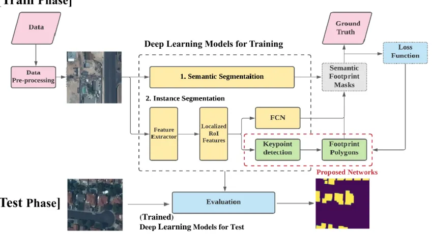
The developed framework employs the typical supervised learning mechanism illustrated in Figure 1.2. The framework is based on a combination of the instance segmentation model with the prediction and grouping of keypoints. The input datasets consist of satellite and aerial images with ground truth annotation of the building footprints, which are regarded as training data. The datasets are preprocessed properly to make them suitable for training deep learning networks for a low computational cost.

The proposed network is based on the instance segmentation approach, which can predict the segmentation mask of each instance extraction through an RPN. Unlike conventional approaches, keypoint detection modules take the place of fully convolutional networks (FCNs), which predict the segmentation mask on localized region-of-interest (RoI) features. The proposed framework is evaluated by comparing its performance against that of two representative models, namely, semantic segmentation and instance segmentation, which are the two axes of deep learning building footprint extraction. The performance is assessed using three metrics, namely, F1 score, interest of union (IoU), and structural similarity index measure (SSIM). For the generalization of model performance, the framework is trained, and the metrics are compared independently on two datasets with different characteristics

６

Figure 1.2. The General Workflow of the Proposed Framework

(Trained)

Deep Learning Models for Test

[Train Phase ]

Deep Learning Models for Training

[Test Phase ]

７

1.2.2 Contribution

The contributions of this thesis are as follows:

 A novel framework for building footprint extraction is proposed by the introduction of a keypoint detection module. Building polygons with improved visibility are obtained by replacing the segmentation task in instance segmentation with keypoint detection.

 The proposed network operates by simply adding the detection network module to the common two-stage instance segmentation networks in end-to-end learning, thereby predicting vectorized building polygons without heavy post-processing algorithm.

 At a satellite image spatial resolution of 30 cm, the proposed keypoint-based building polygon extraction is confirmed to be feasible through experiments and analysis.

８

1.3. Organization of Thesis

The thesis is organized as follows: Chapter 2 reviews relevant works and public dataset for building footprint extraction. Chapter 3 describes the backbone network for building footprint extraction. In Chapter 4, the proposed methodology is explained in three steps, instance segmentation, keypoint estimation and keypoint grouping. Chapter 5 describes the experimental details containing adopted dataset and implementation details for training the networks. Chapter 6 shows experimental results and discussion. Finally, the conclusion of the thesis is given in Chapter 7.

９

Chapter 2. Related Works

2.1. Deep Learning for Object Detection and Semantic Segmentation

2.1.1. Semantic Segmentation

Semantic segmentation classifies the pixels of an image into meaningful classes that are semantically interpretable and correspond to specific categories. An FCN [13] is a typical deep learning model for semantic segmentation, which plays a key role in modern models. The input image is fed into convolutional and pooling layers to extract and interpret the contextual information. The FCN, located at the end of the network, learns from deconvolution layers to upsample the feature map to the original resolution of the image. As this step consists of simply upsampling the score, superior performance is unlikely due to the limited amount of information.

Figure 2.1. U-Net Architecture for Semantic Segmentation [12]

With regard to the structure of FCNs, [14] proposed U-Net, which has an encoder–decoder structure; the encoder part is utilized to capture the context of an image, and the decoder part is utilized to learn the precise localization of the results (Figure 2.1). U-Net also adds a skip connection to the encoder–

decoder structure. Through this skip connection, which directly transfers

１０

information from the contracting path to the expansive path, this model can improve localization performance by reducing information leakage through the networks. Moreover, this model is sensitive to detecting small objects and segmenting densely distributed objects.

2.1.2. Instance Segmentation

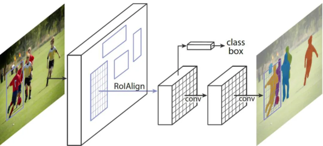
Instance segmentation refers to identifying individual objects and delineating each distinct object of interest. The main approach for this task is Mask R-CNN, whose architecture is shown in Figure 2.2.

Figure 2.2. Mask R-CNN Framework for Instance Segmentation.

Mask R-CNN [15] performs detection and then segmentation. The detection process generates localized RoIs from the feature map from a feature extractor, such as residual network (ResNet) and AlexNet; this feature extractor is the same as the common two-stage object detector (Faster R-CNN) [16, 17]. After this step, the feature of each RoI is fed into simple convolutional layers and an FCN to obtain object masks for semantic segmentation. This approach can be considered a common form of the end-to-end instance segmentation model.

Research has been conducted to improve each module in Mask R-CNN while maintaining the structure of the detection and segmentation modules after a feature extraction [18].

１１

2.2. Building Footprint Extraction

Building footprint extraction is garnering considerable interest as an active field in remote sensing and computer vision research. Established building footprint maps are used in important applications, such as disaster risk management and urban monitoring.

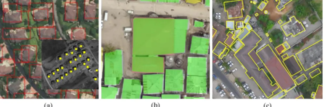
Figure 2.3. Similar Tasks with Building Footprint Extraction: a) Building detection b) Building segmentation c) Building footprint extraction

Building detection and building segmentation are similar to building boundary extraction (Figure 2.3). First, building detection extracts the existence of buildings from a satellite image and performs geometric localization using bounding boxes. It is used in detecting and tracking the number of buildings in a time series image to observe the urban development and disaster response applications¹. Next, building segmentation classifies the pixels occupied by buildings in an image, which include the roofs and visible walls of the buildings [19]. By contrast, building boundary extraction involves the ground boundaries of buildings. Therefore, inconsistencies may occur between the roof boundaries and building footprints from satellite and aerial images. In the case of orthogonal images, such as unmanned aerial vehicle (UAV) and drone images, roof and building boundaries are almost identical. However, for satellite images, the inclination of a building occurs

1 https://spacenet.ai/sn7-challenge/

１２

due to its view angle, and the roof and building boundaries could be inconsistent. Therefore, the above factors should be considered in selecting the training dataset, which will be explained in Section 2.4.

Table 2.1. Categories of Building Footprint Extraction

As shown in Table 2.1, building footprint extraction could be performed through four approaches. Building footprints are often delineated with multistep, bottom-up approaches by using a combination of multispectral satellite and airborne LiDAR imagery [2]. LiDAR data help in localization by using point clouds, which can provide geometrically meaningful information. Building outlines can be obtained by merging convex polygons extracted from the point clouds using a binary space partitioning (BSP) tree.

Satellite images are considered auxiliary data from the LiDAR points to remove trees that are confused with buildings by using the normalized difference vegetation index. Reference [20] generated building footprints by using DTM and DSM estimated from a morphological operator derived from Conventional

method Deep-learning based method

Morphological Operation

Semantic Segmentation

Graph Convolutional Neural Network

Instance Segmentation

 Extract

morphological information such as edges from raw data

 Limitation of the feature to identify building

 Classify each pixel with a corresponding class

 Need additional post-

processing to vectorize

 Calculated the loss between the nodes,

coordinates rather than pixel values

 Significant computational costs

 Combination of detection and segmentation

 Identify each instance of each object

 Can apply Polygonization Module

LiDAR with optical images

Optical

Multispectral Optical RGB Optical RGB

１３

LiDAR data. This approach applies shape optimization algorithms, such as BSP, to extract building boundaries from LiDAR data. Additionally, point cloud data are used for automated 3D building reconstruction and extraction of height information.

2.2.1. Semantic Segmentation

Figure 2.4. General Semantic Segmentation Network for Building Footprint Extraction [21]

A recent approach for building footprint extraction is semantic segmentation, which applies an FCN from a single optical image [5, 6, 21, 22]. Many winning networks in data competitions used multiple convolutional neural networks (CNNs) for semantic segmentation to extract building footprints (Figure 2.4). In particular, the U-Net model, which has an encoder–decoder structure, has been widely used for building extraction and proven effective for solving the binary segmentation problem. Most of the competitors from the SpaceNet 2 and Open Cities AI challenges performed semantic segmentation using ensembles of U-Net with state-of-the-art image classification encoders. The winning network structure of Open Cities AI is the same as that of SpaceNet 2, and the encoder of the model uses state-of- the-art structures, such as EfficientNet and InceptionNet [23, 24]. The use of new encoders helps increase accuracy by using a deep model design and mitigating the scaling problem.

１４

To overcome this issue, probabilistic graph models, such as the conditional random field (CRF) [25], have been proposed to connect convolutional layers at the final layers as a post-processing step. The main concept behind this model is to transform pixel-wise classification into probabilistic inference.

The final prediction is substantially improved to generate precise boundaries from the initial prediction of pixel-wise labels. However, this framework does not extract a sufficient number of features from the images to facilitate effective propagation of information. Reference [26] introduced an automatic building extraction method that integrates a graph convolutional network (GCN) and deep structured feature embedding into an end-to-end workflow.

To accurately describe edge information, [26] proposed GCN frameworks for building segmentation rather than using DCNNs. Similar to graph models, such as CRF, GCN can aggregate the information from neighbor nodes, which allows the model to learn about local structures. The grid-like data can be interpreted as a special type of graph data where the node is on the grid and the number of neighbors is fixed [26]. However, due to its significant computational cost, the GCN approach has been applied only to low- resolution images, such as Planet (5 m), rather than submeter-resolution satellite images [27].

Building footprint extraction performs beyond building segmentation by identifying each instance of each building. The segmentation result is a binary classification map that classifies only buildings and backgrounds, that is, without building objects. The boundary of each building mask is the result of building boundary extraction. Several challenges, such as SpaceNet 2 and SpaceNet 4, require instantiation in post-processing, as shown by using mean average precision (mAP) for evaluation.

１５

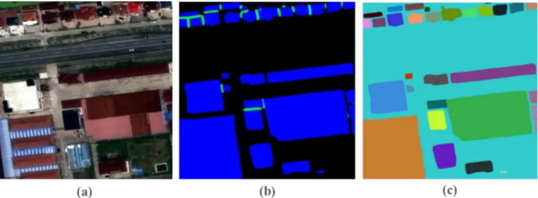
Figure 2.5. Workflow of the Winner’s Algorithm for SpaceNet4 (cannab): a) Input image, b) Segmentation results, blue: building, green: contact points between juxtaposed buildings, c) Instantiation results

Since simple binary segmentation cannot lead to instantiation, SpaceNet 4 challenge winners introduced two additional networks for the division between adjacent buildings, namely, building outline labels and contact points between very closely juxtaposed buildings². As shown in Figure 2.5.b, the proposed network yields three classes, namely, buildings, juxtaposed pixels, and background. The idea of instantiation using the additional adjacent pixels was widely used by various competitors for post-processing that combines the watershed algorithm and LightGBM.

Without post-processing via polygonization, semantic segmentation produces coarse results, such as blurred and rounded boundaries in the output caused by the use of convolutional layers with large receptive fields and pooling layers in DCNNs [28]. A DCNN also fails to use fine local details because it does not consider the interactions between pixels [26]. The lack of local details is significant for refining boundary information (even with the use of post-processing), especially for the detection of small objects which can be obtained as low-level features in satellite images.

2 https://github.com/SpaceNetChallenge/SpaceNet_Off_Nadir_Solutions

１６

Figure 2.6. Polygonization Stage Proposed by Microsoft USBuildingFootprints Benchmarks

As shown in Figure 2.6, the benchmark produced by Microsoft’s building dataset developed post-processing tools separately for polygonization to refine the predicted pixels from segmentation into polygons. Their research was motivated by the Douglas–Peucker algorithm [29], which was manually defined and automatically tuned to impose a priori building properties. For example, the interior angles of the generated polygons must be over 30 degrees so that they are not very sharp, and building angles likely consist of a few dominant angles³.

3 https://github.com/microsoft/USBuildingFootprints

１７

2.2.2. Instance Segmentation

Figure 2.7. Additional Module Based on Single Class Mask R-CNN for Building Footprint Extraction [7]

Instead of generating pixel-wise segmentation maps, instance segmentation approaches were introduced to directly generate polygons in end-to-end networks. This approach is composed of two modules, namely, object detection and vectorization. Polygons are acquired by predicting the optimal locations of the polygon vertices and linking the outer vertices with straight lines, thereby creating formulaic polygons. PolygonRNN [30] and PolygonRNN++ [31] use fully convolutional layers to extract the bounding boxes of each instance; these layers are then fed into sequential recursive neural networks (RNNs), which predict a boundary mask, the locations of the polygon vertices, and the first vertex to start edge generation. In one sequence, the current boundary and vertex prediction are influenced by previous predictions. PolyMapper [9] additionally unifies building footprint extraction and road extraction into a dual pipeline and applies the same network on large-scale aerial images.

Since it is possible to distinguish independent objects, additional modules can be used to enhance the output results, such as reinforcement of edge information with attention modules for extracting effective features [7, 32]

(Figure 2.7). Zhao et al. [3] introduced building boundary regularization,

１８

where polygons are extracted via Mask R-CNN using the minimum description length framework to determine the hypothesis model. This method produces well-regularized polygons through a performance almost equivalent to that of Mask R-CNN. The authors developed the regularization idea by adopting GCNs to conduct polygonization from the extracted vertices.

Zhang et al. [7] directly predicted a point map using FCNs from each proposed RoI. To train the keypoint detector, they used a heatmap indicating the locations of the keypoints. Their study focused on detecting the vertices of an object, not from the segmentation result. Among the extracted keypoints of an object, the extreme keypoint, which is geometrically located on the far left or right, is first selected as the starting point. Then, the object is generated by establishing a connection between it and its nearest neighbor. Through an iterative process, a polygon is formed by uniting all of the edges.

１９

2.3. Keypoints

Keypoint representation is a central component of image matching, retrieval, pose estimation, registration, and 3D reconstruction. Conventional feature detectors localize geometric structures through engineered algorithms, which are often called handcrafted detectors. These keypoint detectors have been extended to handle multiscale and affine transformations. Representatively, SIFT searches for blobs over multiple scale levels and selects stable points as keypoints.

Figure 2.8. Example of Keypoint Detection Results for Classifying Aircraft Type. Keypoints’ Predictions are Marked with Red Dots. [33]

The success of learned methods in general feature descriptors motivated the community to explorer similar ways for feature detectors [34]. FAST [35] was one of the first attempts to use machine learning to predict a corner keypoint detector. With the advance of approaches based on DNNs, global representations have been widely used to solve these problems, as they can be trained in a straightforward, end-to-end manner [12]. Despite the impractical inefficiency of the initial models, CNNs can significantly reduce the errors in local descriptors. Regarding predefined detector anchors, [36]

introduced a new formulation for training neural networks.

Keypoint estimation, such as human pose estimation [37], chair corner point

２０

estimation [38], and aircraft type detection, uses a fully convolutional encoder–decoder structure to predict a heatmap for each type of keypoints [39]

(Figure 2.8). The network is trained through fully supervised learning with L2 loss for a rendered Gaussian heatmap. The training is guided by a multipeak Gaussian heatmap, applying a Gaussian kernel [37].

Keypoints in building extraction are points of interest based on the local image gradient direction, that is, the vertices of a building polygon. SIFT has been used to extract keypoint candidates from urban-area and building detection in satellite images [10]. The neighborhood between different vertices is summarized as edges, and several vertices are grouped together to identify an independent building. PolyMapper [9] deploys keypoint sequence prediction produced by recurrent neural networks for buildings. At each step, an RNN takes the current, revious and first vertex as inputs, and outputs a conditional probability distribution of the vertex next to the current one.

PolyMapper provides compact representation for buildings, but it performs poorly for large buildings due to inaccuracies in its location information.

Reference [40] combined the structure of instance segmentation and FCN- based keypoint estimation networks. However, the ability of the model when applied to satellite images could not be assessed easily because the model was assessed on the Aerial Imagery for Roof Segmentation (AIRS) dataset with a spatial resolution of 0.075 m. Moreover, since the grouping keypoint is adopted by establishing a connection between a vertex and its nearest neighbor, there is a limitation that closed polygons cannot be guaranteed for concave objects.

２１

2.4. Open Datasets for Building Footprint Extraction

Various datasets for building footprint extraction are open to the public for evaluating models. These datasets contain aerial or satellite images with labels annotated as pixel-wise masks or object-wise labels, which refer to the coordinates of the building polygons at the object level. Some widely used datasets are discussed below.

 xBD dataset [41] aims to spur the creation of accurate machine- learning models that assess building damage from pre- and postdisaster satellite imagery. It contains over 5000 km² of RGB satellite images sized 512 × 512 pixels. The image spatial resolution is 50 cm, with satellite images provided from WorldView-2 and GeoEye-1. The annotations are rasterized into a binary mask image, and images are depicted based on a diversity of disasters.

 Microsoft Building Footprints was made by a collaboration between Microsoft Maps & Geospatial teams to provide building footprint extraction labels across the Unites States and Canada. The labels are automatically annotated using the Bing map, and over 136 million footprints were extracted. Unlike in other datasets, the backend of this dataset provides polygonization tools for improved segmentation results.

 AIRS (Aerial Imagery for Roof Segmentation) [42] consists of aerial images from the city of Christchurch, New Zealand, with 7.5 cm RGB bands. The annotations of building roof outlines are carefully refined and aligned in this database. The AIRS database includes over 220,000 buildings with object-wise labels.

 SpaceNet 2 dataset [43] contains 24,586 satellite images of WorldView-3 images for four cities, namely, Las Vegas, Paris, Shanghai, and Khartoum, which have different background complexities and contain a high diversity of building roof styles. The

２２

images are provided in a variety of formats, including panchromatic, 8-band, and pansharpened RGB images. The RGB images are sized 650 × 650 pixels and have a 30 cm resolution. In this database, over 300,000 buildings are annotated with object-wise labels.

 OpenCitiesAI dataset features 7.5-cm-resolution drone imagery from African cities, which contain small and highly diverse building roof styles. The images have a size of 512 × 512 pixels with RGB bands. Building footprints are annotated with the local OSM data.

The database covers more than 700,000 buildings in 12 African cities and regions.

Figure 2.9 Annotation Errors between Roof Outline and Building Boundary

Statistics related to the datasets are summarized in Table 2.2. The ideal building footprint label is an orthorectified image with manually annotations at the roof outlines, but no dataset perfectly meets this condition. Except AIRS, which was annotated manually for building roofs, datasets are automatically annotated using OSM building footprint data. As shown in Figure 2.9.b, there may be bias of misalignment between the roof contour observed in a satellite image and the building footprint, given that the label is only annotated to the building’s ground footprint. This misalignment problem is highlighted in

２３

datasets of satellite images; the larger the building height or view angle, the larger the actual bias. Therefore, in some competitions, such as SpaceNet 4, competitors try to overcome this problem by learning with additional one- hot-encoded information of the view angle or satellite position. However, typically, the larger the view angle, the less the accuracy.

Orthorectified images from UAVs or drones are acquired at nadir angle; thus, they are not affected by the misalignment problem. However, during geometric correction for image mosaicing, the texture of building boundaries may be distorted. In addition, some buildings are often not annotated due to omissions in OSM. Depending on the location where an image was acquired, each dataset has a different background and building roof style. As such, datasets for training should be selected by considering the advantages, disadvantages, and locations of image acquisition.

The SpaceNet 2 and Open Cities AI datasets are chosen in this study to evaluate the proposed model. SpaceNet 2 is the most widely used dataset, winning algorithms from the challenge are highly accessible, and different models for building footprint extraction have been trained on this dataset; thus, it is selected for direct comparison with state-of-the-art models. Since the dataset consists of images from four different continents, the generalization of the model algorithms must be assessed. However, several images, excluding Khartoum, are from rural landscapes and provided as satellite images, whose view angle may affect detection accuracy. The SpaceNet 2 dataset also does not include the building footprint characteristics of developing countries, where buildings are typically small and densely distributed.

In addition, SpaceNet 2, which is composed of satellite images, may exhibit misalignment between the roof contour and the building footprint. Hence, the Open Cities AI dataset, which is based on drone images, is used as auxiliary data for training. The Open Cities AI dataset can compensate for the limitation of SpaceNet 2 in our evaluation of the generalization of the proposed model,

２４

since the dataset includes characteristics of developing countries in Africa.

The dataset also contains orthorectified images with matched roof boundaries and building footprints. However, since the images included in the dataset were geometrically located, any sign of geometric distortion can easily be detected visually. For this reason, many of the teams participating in the challenge decreased the spatial resolution of the original images from 3 to 10 cm. Likewise, we lowered the resolution for the subsequent training phase, but to facilitate direct comparison with the SpaceNet 2 dataset, we downsampled the images to a matching spatial resolution of 30 cm.

Table 2.2. Statistics of the Datasets for Building Footprint Extraction

Dataset xBD Microsoft

Building Footprints

AIRS SpaceNet2 OpenCitiesAI

Year 2019 2019 2019 2018 2020

Type Satellite Aerial Aerial Satellite Aerial

Location Worldwide US, Canada New Zealand

Las Vegas, Paris, Shanghai, Khartoum

12 cities in Africa

Data Type RGB RGB RGB RGB +

8-band RGB

Image Resolution

(cm/pixel) 50 30 7.5 30 3

Image Size

(pixels) 512×512 - - 650×650 -

Annotations 550k 125m 220k 300k 790k

View angle 0~55 orthorectified orthorectified 0~30 orthorectified

２５

Chapter 3. Backbone Network

In this chapter, the backbone network for building footprint extraction is introduced. The backbone network follows the typical two-stage instance segmentation approach proposed from Mask R-CNN. This approach activates to predict segmentation mask, separating the involved tasks into detection and segmentation. This architecture outputs well-localized RoI features, which play a key role in the models in the next chapter.

The backbone network is derived for feature encoding, building detection, and localization. A combination of a ResNet and a feature pyramid network (ResNet-FPN) [44] is utilized to extract deep features at multiple scales. A two-stage object detection approach is employed through the RPN to detect and localize building objects [17], and a fully convolutional layer is used to regress the scale of bounding boxes. An RoIAlign [15] layer is applied to precisely crop the bounding boxes with the feature map, thereby obtaining a well-localized RoI for each object. Localized features are essential for predicting pixel-wise segmentation or keypoint detection. The structure of the backbone network is illustrated in Figure 3.1.

２６

Figure 3.1. Overview of Backbone Network and Proposed Framework

２７

3.1. Feature Extraction

Figure 3.2. Feature Pyramid Networks for Object Detection

As shown in Figure 3.2, feature extraction is the conversion of a given input image into a set of features; this process is involves decreasing the quantity of assets needed to define a large set of information [45]. It is divided into bottom-up and top-bottom pathways. First, the image is input into a five-stage of ResNet (C1–C5); each stage of ResNet consists of several convolution layers and applies 2 × 2 pooling at the last layer to downsample the feature map.

The residual blocks substitute the convolutional blocks to deepen the networks. The top-down part of the network integrates features from different scales generated from the bottom-up part. It first applies a 1 × 1 convolution kernel to the current feature map and adds it element-wise with its upsampled previous feature map. It learns a 3 × 3 convolution to output the feature map, which has different scales (P2–P5).

２８

Detecting objects at different scales is an essential task because the input satellite images cover larger areas and contain various sizes of building objects. The multiscale feature maps obtained from the FPN can detect building objects from different scales, unlike feature maps of only one scale (such as C5).

3.2. Localization

The RPN, which has predefined anchor boxes, generates the initial proposed bounding boxes, which are used to crop the feature maps to obtain the cropped features. RoI pooling is then adopted on the cropped features to obtain RoI features, which are input into the bounding-box regression and classification layer to produce the coordinate and class scores of the refined bounding boxes [15]. Lastly, the multiscale feature maps and the final bounding boxes are fed into the RoIAlign to generate precisely localized RoI features.

3.2.1. Region Proposal Network

The inputs of the RPN are the multiscale feature maps and predefined anchor boxes. These anchor boxes are generated with various sizes and width- to-height ratios for different strides on the input image (Figure 3.3). The RPN will predict bounding-box proposals for the corresponding anchor boxes through a box regression layer and class scores through classification on each entry of the feature maps. The classification layer is designed to distinguish positive and negative boxes, that is, boxes contain objects and empty boxes.

２９

Figure 3.3. Region Proposal Network for Finding out the Possible Locations of the Targets in the Image [17]

The class score of each predicted bounding box is the objectness score. The bounding-box proposals are then filtered through Non Maximum Suppression (NMS) [46] based on a threshold of the objectness score to reduce its total number and to maintain the ratio of the positive and negative proposed boxes (usually 3:1). The box proposals are then closer to the object locations in the image compared with the input anchor.

3.2.2. Localization Layer

The multi-scale feature maps are cropped using the box proposals from the RPN. The feature maps are cropped based on the size of the box proposals according to the following equation:

k = [k₀+ log₂(√𝑤ℎ/224)] (3-1) where w and h are the width and height, respectively, of the box proposal.

k₀ = 4, and k is the level of scale for cropping the feature map. The cropped

３０

features, which are of various scales, are fed into an RoI pooling layer to normalize them into RoI features with a fixed size of 14 × 14 [15]. The cropping operation performs feature scale selection, thus allowing the feature scales to match the size of the detected objects. Hence, feature maps with larger (smaller) resolutions correspond to smaller (bigger) objects.

Identification of such correspondence takes advantage of the multiscale feature maps and can exploit richer and more accurate semantic information from different scales. As in the RPN, in the localization layer, the box regression and classification layer are applied to the RoI features to predict the coordinates and class scores of the bounding boxes. This second localization can further refine the bounding-box proposals generated from the initial bounding-box.

3.2.3. RoIAlign

Figure 3.4. RoIAlign for Getting Precise Bounding Box Prediction[15]

The coordinates of the RoI features are usually floating numbers produced from the box regression layer. The cropping and RoI pooling will simply convert them into integer numbers in a quantization process, thus causing rounding errors and misalignment. As shown by a study on Mask R-CNN [13], simple cropping and RoI pooling are not sufficient for acquiring precisely localized feature maps for pixel-wise segmentation, which requires pixel- level accuracy (Figure 3.4). Therefore, it designs an RoIAlign layer to address

３１

the misalignment problem and improve the accuracy of the RoI features.

Instead of directly taking the integer of the floating RoI coordinates, which is affected by round-off errors in the cropping and RoI pooling, RoIAlign reserves the floating coordinates and uses differentiable bilinear interpolation to obtain the values of the floating points and the final localized RoI features.

3.3. Loss Function

For the training of the entire backbone network, losses should be calculated for the object detection of the two stages of the RPN, namely, box regression and classification. The loss function of the backbone network is the sum of the three types of losses, and it is defined as follows:

𝐿 = 𝐿_𝑐𝑙𝑠+ 𝐿_𝑏𝑜𝑥+ 𝐿_{𝑚𝑎𝑠𝑘} (3-2) As for the classification score loss, a binary cross entropy loss of classification is computed:

𝐿_cls(𝑝(𝑦)) = −(𝑦𝑙𝑜𝑔(𝑝(𝑦)) + (1 − 𝑦) log(1 − 𝑝(𝑦)) (3-3) where y is the predicted class label (0 or 1) and p(y) is the probability score for the class label.

In accordance with Faster R-CNN [15], the box deltas between the predicted box and the ground truth box are calculated as inputs of the box regression loss function rather than the box coordinates. The deltas are defined as follows:

t_x = (𝑥 − 𝑥_𝑎)/𝑤_𝑎, t_y = (𝑦 − 𝑦_𝑎)/ℎ_𝑎,

𝑡_𝑤 = log (𝑤/𝑤_𝑎), 𝑡_ℎ = log (ℎ/ℎ_𝑎) (3-4)

３２

t_x^∗ = (𝑥^∗− 𝑥_𝑎)/𝑤_𝑎, t_y^∗ = (𝑦^∗ − 𝑦_𝑎)/ℎ_𝑎,

𝑡_𝑤^∗ = log (𝑤^∗/𝑤_𝑎), 𝑡_ℎ = log (ℎ^∗/ℎ_𝑎) (3-5) In the equation of the box regression, x and y are the coordinates of the center point of the bounding box, and w and h are its width and height, respectively. x, xa, and x^* are for the predicted, anchor, and ground truth boxes, respectively.

The box deltas (t_x, 𝑡_𝑦, 𝑡_𝑤, 𝑡_ℎ ) are predicted; they are equivalent to the regression from a predefined anchor box to a predicted box. To compare the predicted box deltas with the ground truth (𝑡_𝑥^∗, 𝑡_𝑦^∗, 𝑡_𝑤^∗, 𝑡_ℎ^∗), which represent the regression values from an anchor box to its closest ground truth box, we adopt the smooth L1 loss [47].

𝐿_𝑏𝑜𝑥(𝑡, 𝑡^∗) = ∑ 𝑠𝑚𝑜𝑜𝑡ℎ_𝐿1(𝑡 − 𝑡^∗) (3-6)

The mask loss is defined as the average binary cross-entropy loss, which is a per-pixel sigmoid. The mask branch has an m²-dimensional output for each RoI, which encodes binary masks of a resolution of m².

𝐿_{𝑚𝑎𝑠𝑘} = − 1

m² ∑ [𝑦_𝑖𝑗𝑙𝑜𝑔𝑦_𝑖𝑗^∗ + (1 − 𝑦_𝑖𝑗) log(1 − 𝑦_𝑖𝑗^∗)]

1≤𝑖,𝑗≤𝑚

(3-7)

where y_ij is the ground truth of a pixel (i,j) in the true mask for a region of size m × m. y_ij^∗ is the predicted mask of the same cell in the mask.

３３

Chapter 4. Proposed Network

The framework was designed to develop a segmentation model that can extract building footprints while producing low-complexity, geometry- preserving masks for each building. The proposed architecture combines polygon-based methods with Mask R-CNN (Figure 4.1). In this section, the backbone architecture for the building footprint extraction model is described first. Next, the proposed model is presented, which focuses on capturing the local geometry of the object.

Figure 4.1. The Flowchart of the Proposed Approach for Building Footprint Extraction. FCN: Fully Convolutional Network, conv:

convolutional block.

３４

4.1. Instance Segmentation

The goal of instance segmentation is to provide a segmentation mask for polygon initialization for each individual object. The instance segmentation model is exploited to generate a segmentation mask for each instance in the scene, as in the typical Mask R-CNN. A bounding-box detection step is added to predict separate keypoints and partition the image into individual building instances. ResNet–FPN is integrated for supposing RoIs into the framework [44]. The FPN enhances the performance of the RPN by adding additional information through a multiscale pyramidal hierarchy of CNNs called feature pyramids.

Once bounding boxes of individual buildings are generated, the mask generation pipeline is processed. The pixel-wise mask of the target is predicted from the localized RoI extracted from the FPN. If the object detection model outputs proposal boxes, an FCN branch will be adopted on each RoI feature to predict the class probability of each instance, that is, to estimate a binary classification of buildings and backgrounds (Figure 4.2).

Figure 4.2. FCN Branch to Predict Mask Logits. The Input RoI Feature Fed into Sequential 𝟑 × 𝟑 Convolutional Layers, Batch Normalization and ReLU Layers [15].

The FCN branch consists of several sets of convolutions, batch normalization, and ReLU to learn the mask in addition to one deconvolutional layer to increase the resolution. At the end of the pipeline, a sigmoid activation layer is added to produce pixel-wise mask logits, which are used to compute the segmentation loss. The channel of the mask logits is 2, representing the probabilities for the foreground (building) and background

３５

with respect to each pixel. A threshold of 0.5 is used to generated a binary mask from the foreground mask, which can be obtained from the pixel-wise segmentation of the building masks.

３６

4.2. Keypoint Estimation

Figure 4.3. Input Image with Annotation and Its Keypoint Heatmap

The keypoint estimation step outputs a heatmap of keypoints for each object.

The proposed keypoint prediction network is similar to that in [48]. Let 𝐼 ∈ ℛ^{𝐻×𝑊×3} be an input image of height H and width W. For each image patch, there exists a corresponding ground truth heatmap such that 𝑌 ∈ [0,1]^𝐻×𝑊. The aim of this process is to produce a corresponding heatmap of candidate keypoints, 𝑌̌ ∈ [0,1]^𝐻×𝑊 , which represents the vertices of each instance (Figure 4.3). A prediction 𝑌̌ = 1 corresponds to a detected keypoint, while 𝑌̌ = 0 denotes the background.

For each ground truth keypoint 𝑝 ∈ ℛ², the ground truth keypoint map is guided by using the Gaussian kernel Y_𝑥,𝑦 = exp (−^{(𝑥−𝑝𝑥)}

2+(𝑦−𝑝𝑦)²

2𝜎_𝑝² ), where 𝜎_𝑝² is an object size-adaptive standard deviation [48]. In this regard, the penalty is reduced to negative locations within a radius of the positive location instead of applying equal penalization during training [7]. Therefore, the training object is set as a penalty-reduced pixel-wise logistic regression with modified focal loss to maintain a balance between positive and negative locations [49]. An example of the heatmap generation result is shown in

３７

Figure 4.3.

𝐿_{𝑘𝑒𝑦𝑝𝑜𝑖𝑛𝑡}

= −1

𝑁∑ {(1 − 𝑌̌_𝑥𝑦)^𝛼log(𝑌̌_𝑥𝑦) 𝑖𝑓 𝑌_𝑥𝑦 = 1 (1 − Y_𝑥𝑦)^𝛽(𝑌̌_𝑥𝑦)^𝛼log(1 − 𝑌̌_𝑥𝑦) 𝑜𝑡ℎ𝑒𝑟𝑤𝑖𝑠𝑒

𝑥𝑦

(4-1)

where 𝛼 and 𝛽 are hyper-parameters for focal loss and N is the number of objects in a patch. For this study, the hyper-parameters are fixed as 𝛼 = 2 and 𝛽 = 4, in accordance with [49].

Figure 4.4. Mask and Keypoint Branches

Segmentation masks are regarded as a rough probability map that estimates the probability of each pixel belonging to the foreground or not [50, 51]. With the merging of the segmentation masks with the feature inside an RoI, the mask can be used to distinguish whether a keypoint is enclosed inside of an object or not (Figure 4.4). Then, the FCN is applied to the local features acquired by RoIAlign with the predicted mask to predict the heatmap of the keypoints.

Overall, the total loss function of the proposed network is a multitask loss function expressed as follows:

３８

L = Lcls+ 𝐿𝑟𝑒𝑔+𝜆_{𝑚𝑎𝑠𝑘}𝐿_{𝑚𝑎𝑠𝑘}+ 𝜆_{𝑝𝑜𝑙𝑦𝑔𝑜𝑛}𝐿_{𝑝𝑜𝑙𝑦𝑔𝑜𝑛} (4-2) where L_𝑐𝑙𝑠 is a cross-entropy loss for bounding-box classification and 𝐿_𝑟𝑒𝑔 is a bounding-box loss for bounding-box regression, which is defined in [15].

For all experiments in this study, 𝜆_{𝑚𝑎𝑠𝑘} = 0.2 and 𝜆_{𝑝𝑜𝑙𝑦𝑔𝑜𝑛} = 1 unless specified otherwise. The features of the backbone are passed through a separate 3 × 3 convolution, ReLU, and 1 × 1 convolution.

３９

4.3. Grouping Keypoints

Figure 4.5. Strategy for Grouping Keypoints

To create a polygon where edges are sequentially connected with keypoints, a simple geometric method is adopted for the predicted keypoints (Figure 4.5).

First, four extreme keypoints, located at the farthest left, right, bottom, or top of an instance, are selected as the group of the start point. Then, a Euclidean distance matrix of all keypoints is calculated to search for the distance connecting the extreme keypoints. The point with the shortest distance with respect to an extreme point is first selected as the start point, and the first edge is generated by establishing a connection between this initial point and its extreme point. Then, the generated point is considered the initial point for creating the next polygon; the next set of vertices is connected with those in its neighborhood. The grouping of keypoints is iterated until the final keypoint meets the initial keypoint. Finally, a polygon of an object is formed by integrating all of the generated edges. One limitation occurs when the shape of a ground truth object is concave; the grouping method fails to utilize all keypoints to create a complete polygon. This problem can be resolved by establishing a connection between the initial point and its next closest point.

４０

Chapter 5. Experimental Design

In this chapter, the result of the proposed framework (introduced in Chapter 3) is presented. Section 4.1 introduces the characteristics of the data used to evaluate the models. Section 4.2 presents the experiments from data acquisition and pre-processing implementation of the network models to the training process and details.

5.1. Data Characteristics

SpaceNet 2 is one of the datasets utilized in this study for the evaluation of the proposed framework. The SpaceNet 2 dataset was distributed through the building footprint extraction challenge at the Conference on Computer Vision and Pattern Recognition (CVPR) 2018. The dataset contains high-resolution satellite images and ground truth for the building footprints. These images are from four cities (Las Vegas, Paris, Shanghai, and Khartoum) covering both urban and suburban regions. The dataset thus includes data with dissimilar characteristics. Each city is associated with four different continents, showing the high diversity of the dataset’s characteristics, specifically with regards to the building roofs and landscape backgrounds. Sample images are shown in Figure 4.1. The images were captured by using the WorldView-3 satellite at a spatial resolution of 30 cm. Due to the non-nadir viewing angle, the roof boundaries and building footprints do not match accurately. The image size is 650 × 650, which is equal to an area of 200 m × 200 m. The total SpaceNet 2 dataset includes 24,587 satellite images with 302,701 building footprints.

The Open Cities AI dataset is also used in this study to evaluate the proposed framework. The dataset was provided by Open Cities AI Challenge:

Segmenting Buildings for Disaster Resilience, which was hosted by the Global Facility for Disaster Reduction and Recovery. The images were acquired by using a drone with a spatial resolution of 7.5 cm to capture images

４１

from Africa. The images contain small, highly diverse building roof styles.

Unlike the SpaceNet 2 dataset, which consists of non-nadir satellite images, Open Cities AI contains orthorectified images. Hence, the roof boundaries and building footprints match correctly. However, since the labels were annotated automatically through OSM, the ground truth has omission errors.

The entire dataset contains over 790,000 building footprint labels. Examples of images and annotations from both datasets are shown in Figure 5.1.

４２

Figure 5.1. Sample Images of SpaceNet2 and OpenCitiesAI at the Four Different Sites.

４３

5.2. Implementation Details 5.2.1. Data Pre-processing

SpaceNet 2 provides several types of satellite images, namely, multispectral, panchromatic, pansharpened multispectral, and pansharpened RGB images.

The pansharpened RGB images were selected for this study’s experiments, as the 3-band input enables the loading of pretrained weights for feature extractors, such as ResNet.

1) Each raw image has a radiometric resolution of 16 bits, so the resolution was converted to 8-bit, similar to that of a natural image. A two percent clip of each image’s histogram was processed to improve the visual interpretation of the image.

2) The annotations of the building footprint labels are provided in GeoJSON format for each image. The annotations are specified with the following names: ImageId, BuildingId, PolygonWKT-Pix, and PolygonWKT-Geo. ImageId and BuildingId specify the unique identity of the images and building instances, respectively. PolygonWKT-Pix and PolygonWKT-Geo denote the coordinates of building polygon vertices in the image space (x,y) and the geographic space (latitude, longitude). The annotation PolygonWKT-Geo was deleted to convert the GeoJSON format to JSON..

3) The GeoJSON files were merged into one JSON file, in accordance with the COCO format [52]. For each object, the minimum and maximum coordinates (𝑥_𝑚𝑖𝑛, 𝑦_𝑚𝑖𝑛, 𝑥_𝑚𝑎𝑥, 𝑦_𝑚𝑎𝑥) were identified and added to the collection of annotations.

4) The images were reshaped from 650 × 650 to 512 × 512 to modify the original images into a suitable size for common instance segmentation tasks. The original images were first upsampled using bicubic interpolation to produce 1024 × 1024 images. Then, these images were split into four 512 × 512 patches to minimize the

４４

computational cost.

5) After pre-processing, the data for each city were divided into 70%

training, 15% validation and 15% testing sample sets.

The Open Cities AI dataset features 7.5-cm-resolution drone images sized greater than 30,000 × 30,000 and in GeoTIFF data format. The annotation format of the GeoJSON files was converted to standard COCO for