저작자표시-비영리-변경금지 2.0 대한민국 이용자는 ... - S-Space

(1)

저작자표시-비영리-변경금지 2.0 대한민국 이용자는 아래의 조건을 따르는 경우에 한하여 자유롭게

l 이 저작물을 복제, 배포, 전송, 전시, 공연 및 방송할 수 있습니다. 다음과 같은 조건을 따라야 합니다:

l 귀하는, 이 저작물의 재이용이나 배포의 경우, 이 저작물에 적용된 이용허락조건 을 명확하게 나타내어야 합니다.

저작권법에 따른 이용자의 권리는 위의 내용에 의하여 영향을 받지 않습니다. 이것은 이용허락규약(Legal Code)을 이해하기 쉽게 요약한 것입니다.

Disclaimer

저작자표시. 귀하는 원저작자를 표시하여야 합니다.

비영리. 귀하는 이 저작물을 영리 목적으로 이용할 수 없습니다.

변경금지. 귀하는 이 저작물을 개작, 변형 또는 가공할 수 없습니다.

(2)

i

공학석사학위논문

자율주행을 위한 정지 장애물 맵과 GMFT 융합 기반 이동 물체 탐지 및 추적

Detection and Tracking of Moving Object based on Interaction of Static Obstacle Map and Geometric Model-

Free Tracking for autonomous driving

2019년 8월

서울대학교 대학원

기계항공공학부

윤 정 식

(3)

i

Abstract

Detection and Tracking of Moving Object based on Interaction of Static Obstacle Map and Geometric Model- Free Tracking for autonomous driving

YOON JEONG SIK School of Mechanical and Aerospace Engineering The Graduate School Seoul National University

Based on the high accuracy of LiDAR sensor, detection and tracking of moving objects(DATMO) have been advanced as an important branch of perception for an autonomous vehicle. However, due to crowded road circumstances by various kind of vehicles and geographical features, it is

(4)

ii

necessary to reduce clustering fail case and decrease the computational burden.

To overcome these difficulties, this paper proposed a novel approach by integrating DATMO and mapping algorithm. Since the DATMO and mapping are specialized to estimate moving object and static map respectively, these two algorithms can improve their estimation by using each other’s output. Whole perception algorithm is reconstructed using feedback loop structure includes DATMO and mapping algorithm. Moreover, mapping algorithm and DATMO are revised to innovative Bayesian rule-based Static Obstacle Map(SOM) and Geometric Model-Free Tracking(GMFT) to use each other’s output as the measurements of filtering process. The proposed study is evaluated via driving dataset collected by vehicles with RTK DGPS, RT-range and 2D LiDAR.

Several typical clustering fail cases that had been observed in existing DATMO approach are reduced and code operation time over the whole perception process is decreased. Especially, estimation of moving vehicle’s state include position, velocity, and yaw angle show less error with references which are measured by RT-range.

Keywords: LiDAR, mapping, Static Obstacle Map, Detection and Tracking of Moving Object, Geometric Model-Free Tracking, Bayesian rule

Student Number: 2017-27903

(5)

iii

4.1 Prediction of target state ... 18

(6)

iv

4.2 Track management ... 19

4.3 Measurement update of target state ... 21

Chapter 5 Experimental Results ... 23

5.1 Vehicles and sensors configuration ... 24

5.2 Detection rate of moving object ... 27

5.3 State estimation accuracy of moving object ... 31

5.4 Code operation time ... 34

Chapter 6 Conclusion and Future Work ... 36

6.1 Conclusion ... 36

6.2 Future works ... 37

Bibliography ... 39

초 록 ... 43

(7)

v

List of Figures

Fig. 1 Structure of proposed integrated perception module with the interaction of DATMO and mapping algorithm. ···6 Fig. 2 (a) Green is LiDAR raw data(Y[k]), gray means grid satisfies

P(𝑥̂_{𝑠𝑡𝑎𝑡𝑖𝑐}^𝑗 [k] = 1) > 0.8 , blue is moving target {𝑥̂_𝑛[𝑘], 𝑍̂_𝑛[𝑘]}

from DATMO. (b) Probability of corresponding grid is occupied static, which means static obstacle map. ··· 11 Fig. 3 Prediction of SOM by the relationship between local coordinate of

current and previous step. ··· 13 Fig. 4 Newly defined measurement 𝑧_{𝑠𝑡𝑎𝑡𝑖𝑐} of motion state of each grid

based on point classification of DATMO. ··· 14 Fig. 5 Local, global coordinate for GMFT and relationship between hunter

and target vehicle using RT range ··· 18 Fig. 6 The measurement of n-th track from corresponding cluster and its

(8)

vi

matching process. ··· 22

Fig. 7 Sensor configuration. ··· 25

Fig. 8 FOV and detection limit of LiDAR··· 26

Fig. 9 Improvement of fail case – Parking lot ··· 27

Fig. 10 Improvement of fail case – Median separator ··· 27

Fig. 11 Evaluation of detection rate with complex traffic, at Nambu- Beltway. Actual moving targets are labeled by manually, and black arrows are detected moving target through proposed approach. Blue means cluster of tracks, green is LiDAR point cloud, gray is SOM. ··· 29

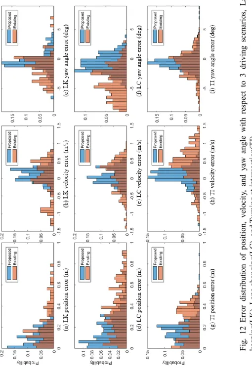
Fig. 12 Error distribution of position, velocity, and yaw angle with respect to 3 driving scenarios, Lane keeping(LK), Lane changing(LC), and Turning at intersection(TI). ··· 32

(9)

vii

List of Tables

Table 1 Detection result of moving vehicles and evaluation by three performance indicators ··· 30 Table 2 Estimation accuracy of main states ··· 33 Table 3 Code operation time of sub-function ··· 35

(10)

viii

Abbreviations

SOM Static Obstacle Map

DATMO Detection and Tracking of Moving Object GMFT Geometric Model-Free Tracking

RTK Real Time Kinematic

SLAM Simultaneous Localization and Mapping OGM Occupancy Grid Map

ICP Iterative Closest Point EKF Extended Kalman Filter

(11)

Chapter 1. Introduction

1

Chapter 1

Introduction

Establishing an accurate and robust perception algorithm using sensor information is essential to develop autonomous driving systems. Among the various sensors, LiDAR has been widely used due to its own characteristics such as high position accuracy. Thus, over the last years, many perception researches have been studied using LiDAR point cloud data as measurement and these researches are often divided into two categories. First is detection and tracking of moving objects(DATMO). Second is mapping method, which has been studied mainly in the field of robotics.

(12)

2

DATMO can be referred to as a process concerned with the states of objects that the robot or autonomous vehicle perceives in a dynamic environment. DATMO algorithm can be categorized according to the objective function that they purpose to optimize, or by the way in which they process the LiDAR point cloud data. Despite all these diversities, what it has in common is that DATMO estimates current states of moving targets and their respective trajectories based on their previously estimated states and the current scan of measurements, usually LiDAR point cloud.

Mapping method is a representative algorithm for implementing environmental mapping. This approach assumes the environment as static, i.e.

having only non-moving objects. Dynamic objects are regarded as noise sources. Recently, mapping is usually conducted through SLAM algorithm.

Based on the assumption that the environment does not transform, SLAM estimates map and location simultaneously. However, this hypothesis is acceptable in some scenarios, but in most real-world environments where dynamic objects cannot be avoided, these approaches encounter errors reducing the overall map quality.

As such, DATMO and mapping method focuses on different issues, state estimation of moving target and construction of static object map respectively, to perceive the world. Even though both are effective algorithms for perceiving surrounding environment, they often show failure in urban autonomous driving

(13)

3

situation when they applied independently. Vehicles in urban road meet various kind of object include static obstacles such as poles, buildings, and parked vehicles. This causes computational load in DATMO algorithm and reduces the quality of clustering, which is sub-function of DATMO for classifying LiDAR point of each target into the same bunch. Furthermore, the mapping method basically assumes that the world is static, which means ego vehicles consider the map never transform, thus the map result from this is distorted by any moving object.

Some works have been conducted to simultaneously solve the SLAM and DATMO using LiDAR. However, detection accuracy and operation time are not presented ([1, 2]) or some paper showed solving two problems at the same time is too demanding due to computation load ([3]). Recently, SLAM in Dynamic Environments (SLAMIDE) has been studied, but following questions are still not solved: How to distinguish between static and dynamic objects, and how to track dynamic objects and predict their position ([4, 5, 6, 7]).

Therefore, this paper proposes a novel approach to improve the estimation accuracy of moving targets and satisfy real-time operation based on the complementary property between DATMO and mapping. Two algorithms are combined into one integrated perception module. Data from each algorithm are used by another algorithm as input or measurement, constructing feedback loop structure.

(14)

4

DATMO and Mapping are not specific algorithms, but rather terms that classify perception algorithms in similar ways. Many algorithms have been proposed to implement each. In this study, GMFT was selected as the DATMO method. This helps to estimate and track a bunch of points without any assumption of the shape of a vehicle. New static obstacle map method also has been directly devised for mapping. Details are given in sections 3 and 4.

The paper is organized as follows: In section 2, concrete structure of interaction between DATMO and mapping algorithm is presented. In section 3, mathematical process of the mapping expanded by the dynamic information of each grid using the Bayesian rule. This dynamic information results from DATMO. Details about the DATMO and its feedback input from the mapping module are shown in section 4. Finally, the experiment in section 5 demonstrates the improvements in the proposed integrated perception module by driving data.

(15)

Chapter 2. Interaction of Mapping and DATMO

5

Chapter 2

Interaction of Mapping and DATMO

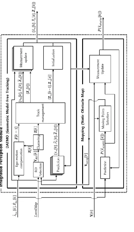
Figure 1 presents proposed integrated perception algorithm. Some main variables that play an important role in this algorithm are displayed. Inputs of the algorithm are states consist of ego vehicle's position, velocity (𝑥̂_{ℎ𝑜𝑠𝑡}[k]), its covariance (𝑃̂_{ℎ𝑜𝑠𝑡}[k]), and Y[k], which is raw data of LiDAR point cloud.

(16)

6

Fig. 1 Structure of proposed integrated perception module with the interaction of DATMO and mapping algorithm.

(17)

7

Outputs, the most important value in this algorithm, are P(𝑥̂_{𝑠𝑡𝑎𝑡𝑖𝑐}^𝑗 [k]) called static obstacle map(SOM) and 𝑥̂_𝑛[𝑘]. The whole space is divided into a grid with side length 𝑑_{𝑔𝑟𝑖𝑑}. 𝑥̂_{𝑠𝑡𝑎𝑡𝑖𝑐}^𝑗 [k] refers to the state of j-th grid at time step k. This is a candidate for 0 or 1 according to whether the corresponding grid is occupied by static objects or not. Thus, if j-th grid is more likely to be occupied by static object than moving object or free space, P(𝑥̂_{𝑠𝑡𝑎𝑡𝑖𝑐}^𝑗 [k] = 1) would be over 0.5 and close to 1, and in the opposite case, P(𝑥̂_{𝑠𝑡𝑎𝑡𝑖𝑐}^𝑗 [k] = 1) would be lower than 0.5 and close to 0. This is applied to all grid in the whole space as the j changes. In general, {𝑥̂_𝑛[𝑘], 𝑍̂_𝑛[𝑘]}, set of each moving vehicles are named track. 𝑍̂_𝑛[𝑘] are clusters of moving vehicles and their states, covariance are 𝑥̂_𝑛[𝑘], 𝑃̂_𝑛[𝑘]. Now, we have all values we want to know from this research. Key concept of this integrated perception algorithm is the interaction between mapping and DATMO. As illustrated between two modules in figure 1, they exchange their output or interim data with each other.

Following are 3 major steps of algorithm.

(1) Mapping module is started by prediction of SOM P(𝑥̅_{𝑠𝑡𝑎𝑡𝑖𝑐}^𝑗 [k]) . By comparing with P(𝑥̅_{𝑠𝑡𝑎𝑡𝑖𝑐}^𝑗 [k]) and Y[k] , tentative moving points Y_{𝑚𝑜𝑣𝑖𝑛𝑔}[k] is selected and delivered to DATMO module. It will be

(18)

8 covered in detail at section 3.1.

(2) Clustering, sub-function that sorts points from one target into the same categories, classifies Y𝑚𝑜𝑣𝑖𝑛𝑔[k] into cluster 𝑍[𝑘]. Comparing it with existing track {𝑥̅_𝑛[𝑘], 𝑍̅_𝑛[𝑘]}, 𝑍[𝑘] are assigned to existing 𝑍̅_𝑛[𝑘] or generate new track 𝑍_𝑛[𝑘] . Lastly, iterative closest point (ICP) and extended Kalman filter (EKF) estimate 𝑥̂_𝑛[𝑘]. More concrete process is discussed at section 4.

(3) Through the DATMO, motion state of all Y[k] points are classified into static, moving, and unknown. SOM is updated using motion state of the corresponding grid, which is calculated based on the result of DATMO.

This measurement update process is conducted through newly devised Bayesian rule which will be covered more detail at section 3.2.

(19)

Chapter 3. Mapping – Static Obstacle Map

9

Chapter 3

Mapping – Static Obstacle Map

Static obstacle map refers to all static objects around of ego vehicle. The whole space is divided into the square-shape grid of which the side is 𝑑_{𝑔𝑟𝑖𝑑}, which is a tuning variable. It seems like this SOM approach is identical with occupancy grid map(OGM) in the mobile robotics, which is a foundation of grid-based SLAM, but it is different from the OGM approach in some manners.

(20)

10

OGM considered the whole map only on the global coordinate, while SOM interprets all LiDAR point cloud data on the local coordinate of ego vehicle.

Each grid of SOM has its own probability of static objects exist in it (P(𝑥̂_{𝑠𝑡𝑎𝑡𝑖𝑐}^𝑗 [k] = 1)). This probability is predicted and updated at every time step k. Figure 2(b) shows a visualization of SOM for all grid in the local coordinate by histogram method. The closer the color is to yellow, the closer the value is to 1. It means that the corresponding grid is more likely to be occupied by static obstacles such as sidewalks, poles, buildings or parked vehicles. It is easily confirmed that the blue clusters of two moving vehicles in front of ego vehicle in figure 2-(a) are eliminated by the proposed integrated perception algorithm in figure 2-(b).

(21)

11

3.1 Prediction of SOM

Since SOM is generated on local coordinate, it needs to be predicted considering consecutive ego vehicle’s motion. The process, which corresponds to time update in Kalman filter, is shown in figure 3. The red and black grid represent previous and current SOM, respectively. Geometric relationship Fig. 2 (a) Green is LiDAR raw data(Y[k]), gray means grid satisfies P(𝑥̂_{𝑠𝑡𝑎𝑡𝑖𝑐}^𝑗 [k] = 1) > 0.8 , blue is moving target {𝑥̂_𝑛[𝑘], 𝑍̂_𝑛[𝑘]} from DATMO. (b) Probability of corresponding grid is occupied static, which means static obstacle map.

(22)

12

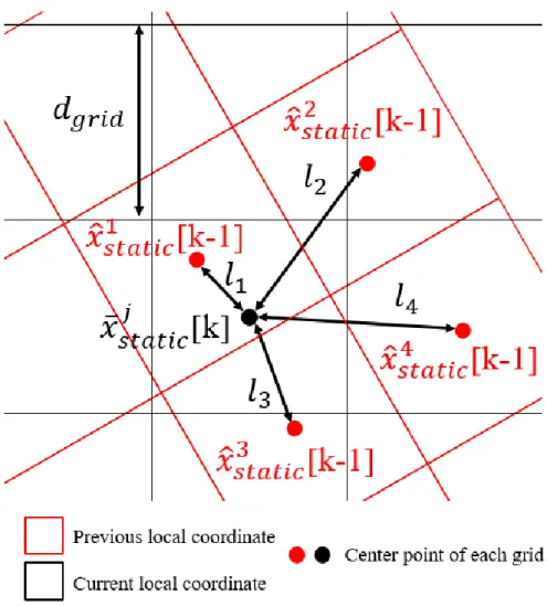
between them can be calculated precisely through a simple transformation matrix since the velocity and yaw rate of ego vehicle is measured and logged by chassis sensor in real time. Four grids of previous SOM enclose the j-th grid of current SOM should be considered to calculating probability of current SOM.

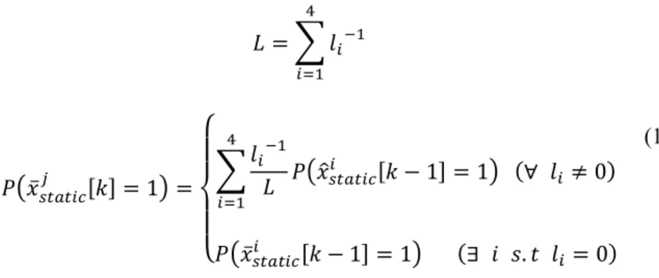
Figure 3 shows these geometric process intuitively. The midpoint of j-th grid of current SOM is 𝑙_𝑖 away from each i-th grid of previous SOM. Therefore, predicted probability of j-th grid is weighted average with weighting factor 1 𝑙⁄_𝑖, which is reasonable since nearby grid should more influence. If any 𝑙_𝑖 is zero, the probability of previous grid is the same with current grid. The process so far is summarized in the following formula (1).

𝐿 = ∑ 𝑙_𝑖⁻¹

4

𝑖=1

𝑃(𝑥̅_{𝑠𝑡𝑎𝑡𝑖𝑐}^𝑗 [𝑘] = 1) =

{

∑𝑙𝑖−1

𝐿 𝑃(𝑥̂_{𝑠𝑡𝑎𝑡𝑖𝑐}^𝑖 [𝑘 − 1] = 1)

4

𝑖=1

(∀ 𝑙_𝑖 ≠ 0)

𝑃(𝑥̅_{𝑠𝑡𝑎𝑡𝑖𝑐}^𝑖 [𝑘 − 1] = 1) (∃ 𝑖 𝑠. 𝑡 𝑙_𝑖 = 0) (1)

(23)

13

Fig. 3 Prediction of SOM by the relationship between local coordinate of current and previous step.

(24)

14

3.2 Measurement update of SOM

Measurement update of SOM updates probability of the static obstacles exist in the corresponding grid(P(𝑥̅_{𝑠𝑡𝑎𝑡𝑖𝑐}^𝑗 [k] = 1)) using measurement 𝑧_𝑛. In this paper, measurement 𝑧_𝑛 is defined by DATMO based on the method shown in figure 4.

As already shown in figure 1, DATMO classifies LiDAR point cloud into moving point, static point and unclassified. These motion states of point cloud Fig. 4 Newly defined measurement 𝑧_{𝑠𝑡𝑎𝑡𝑖𝑐} of motion state of each grid based on point classification of DATMO.

(25)

15

are passed to measurement update of SOM. Green, black, blue points in the left of figure 4 indicate unclassified, moving, static point, determined by DATMO module. As detailed in the right side of figure 4, each grid is classified into 4 categories according to the motion state of point cloud in itself. As a result, each j-th grid is assigned newly defined measurement 𝑧_{𝑠𝑡𝑎𝑡𝑖𝑐}^𝑗 : 𝑧_{𝑠𝑡𝑎𝑡𝑖𝑐}^𝑗 = 0 represents free grid, 1 for unclassified grid, 2 is moving grid and 3 is static grid.

After the measurement of each grid(𝑧_{𝑠𝑡𝑎𝑡𝑖𝑐}^𝑗 ) is determined by the above description, the SOM is updated by the following Bayesian rule using predicted SOM and the likelihood of measurement 𝑧_{𝑠𝑡𝑎𝑡𝑖𝑐}^𝑗 .

SOM for all j-th grid 𝑃(𝑥̂_{𝑠𝑡𝑎𝑡𝑖𝑐}^𝑗 [𝑘] = 1) is calculated through following formula (2), based on the motion state of corresponding grid, 𝑧_{𝑠𝑡𝑎𝑡𝑖𝑐}^𝑗 [𝑘]. 𝑟 is assigned one of the value among 0, 1, 2, 3, which indicate the motion state of each grid, as mentioned above.

𝑃(𝑥̂_{𝑠𝑡𝑎𝑡𝑖𝑐}^𝑗 [𝑘] = 1|𝑧_{𝑠𝑡𝑎𝑡𝑖𝑐}^𝑗 [𝑘] = 𝑟)

= 𝑃(𝑧_{𝑠𝑡𝑎𝑡𝑖𝑐}^𝑗 [𝑘] = 𝑟|𝑥̅_{𝑠𝑡𝑎𝑡𝑖𝑐}^𝑗 [𝑘] = 1)𝑃(𝑥̅_{𝑠𝑡𝑎𝑡𝑖𝑐}^𝑗 [𝑘] = 1)

∑_𝑖=0,1𝑃(𝑧_{𝑠𝑡𝑎𝑡𝑖𝑐}^𝑗 [𝑘] = 𝑟|𝑥̅_{𝑠𝑡𝑎𝑡𝑖𝑐}^𝑗 [𝑘] = 𝑖)𝑃(𝑥̅_{𝑠𝑡𝑎𝑡𝑖𝑐}^𝑗 [𝑘] = 𝑖) 𝑃(𝑥̂_{𝑠𝑡𝑎𝑡𝑖𝑐}^𝑗 [𝑘] = 1) = 𝑃(𝑥̂_{𝑠𝑡𝑎𝑡𝑖𝑐}^𝑗 [𝑘] = 1|𝑧_{𝑠𝑡𝑎𝑡𝑖𝑐}^𝑗 [𝑘] = 𝑟) 𝑖𝑓 𝑧_{𝑠𝑡𝑎𝑡𝑖𝑐}^𝑗 [𝑘] = 𝑟 𝑓𝑜𝑟 𝑟 = 0, 1, 2, 3

(2)

(26)

Chapter 4. DATMO – Geometric Model-Free Tracking

16

Chapter 4

DATMO – Geometric Model- Free Tracking

In this section, Geometric Model Free Tracking (GMFT) will be explained in detail. GMFT uses the non-static points extracted from SOM to track the moving objects and estimate its state. Through this process, it is possible to construct correspondences of non-static points in the consecutive scan and to update the SOM by estimating the motion state of each point based on this

(27)

17

correspondence. In our approach, unlike the previous studies, each point is treated dependently via clustering using Euclidean distance. Since the correspondence between points is derived based on the distance between the mean points of the cluster and the similarity of shape, it is possible to establish the correspondence between points in consecutive scans even with a small calculation. After establishing the correspondence, the matching using ICP is performed for each cluster, and the states of the moving objects are estimated through the EKF using the moving distance and direction of the cluster mean.

GMFT uses two coordinates, which are shown in figure 5. 𝑋_𝐺𝑌_𝐺 is a fixed global coordinate system and 𝑋_𝐿𝑌_𝐿 is a local moving coordinate system that moves with the rear axle of the ego vehicle. There are seven states 𝑥 = [𝑝_𝑛,𝑥, 𝑝_𝑛,𝑦, 𝜃_𝑛, 𝑣_𝑛,𝑥, 𝛾_𝑛, 𝑎_𝑛,𝑥, 𝛾̇_𝑛] and one cluster (𝑍̅_𝑛, 𝑍̂_𝑛) for expressing the n- th track. {𝑝_𝑛,𝑥, 𝑝_𝑛,𝑦} represent the mean position of the cluster respect to 𝑋_𝐿𝑌_𝐿. After completing measurement update at every step, if the cluster point configuration changes, it is replaced with the new mean point. 𝜃_𝑛 means the yaw angle of the moving object respect to 𝑋_𝐿𝑌_𝐿. 𝑣_𝑛,𝑥 means the velocity in the direction respect to 𝑋𝐿𝑌𝐿 . 𝛾𝑛, 𝑎𝑛,𝑥 , and 𝛾̇𝑛 represent yaw rate, acceleration, and angular acceleration respect to 𝑋_𝐺𝑌_𝐺 , respectively. 𝑣_𝑥, 𝛾 represent velocity and yaw rate of ego vehicle at 𝑋_𝐺𝑌_𝐺, respectively. 𝑍̅_𝑛, 𝑍̂_𝑛 denote the predicted cumulative cluster and the updated cumulative cluster of n-th track, respectively.

(28)

18

4.1 Prediction of target state

The prediction of each track is conducted by discretizing the model (3).

Discretization has been done up to the second order, and details are given in [8].

The difference from the references is how to update each point of the cluster.

In this study, (3) is applied independently for all points, assuming that the points in the same cluster have the same state except position. In this case, the shape of clusters can be changed theoretically, but it does not have a significant effect on the actual situation because it predicts only the measurement interval of 80 msec (Frequency of IBEO LiDAR is 12.5Hz).

It is necessary to convert the clusters at previous step to local coordinate 𝑋_𝐿𝑌_𝐿 of current step to initialize the tracks and to estimate the velocity of moving objects. This process is referred to as Ego-motion compensation in Fig. 5 Local, global coordinate for GMFT and relationship between hunter and target vehicle using RT range

(29)

19

figure 1 and only used in order to initialize new track. The clusters of the previous step (𝑍[𝑘 − 1]) are converted to clusters of the local coordinate at current step(𝑍̅[𝑘 − 1]) using dead reckoning via velocity and yaw rate of ego vehicle under the static assumption.

𝑥̇_𝑛= 𝑓(𝑥_𝑛, 𝑢) + 𝑞 = [𝑓₁ 𝑓₂ 𝑓₃ 𝑓₄ 𝑓₅ 𝑓₆ 𝑓₇]^𝑇+ 𝑞 u = [𝑣_𝑥, γ], 𝑞~𝑁(0, 𝑄)

𝑓₁= 𝑣_𝑛,𝑥𝑐𝑜𝑠𝜃_𝑛− 𝑣_𝑥+ 𝑝_𝑛,𝑦𝛾 𝑓₂= 𝑣_𝑛,𝑥𝑠𝑖𝑛𝜃_𝑛− 𝑝_𝑛,𝑥𝛾 𝑓₃= 𝛾_𝑛− γ, 𝑓₄= 𝑎_𝑛,𝑥 𝑓₅ = 𝛾̇_𝑛, 𝑓₆= −𝑘_𝑎, 𝑓₇= −𝑘_𝛾̇

(3)

4.2 Track management

Track management is a task that assigning the clusters of current step to the predicted tracks, generating new tracks using clusters not assigned to the any predicted tracks, and removing the tracks that have not been updated for a certain period. The assignment of the clusters to the predicted track is performed via Global Nearest Neighbor (GNN). For a detailed description of track management, we need to explain the meaning of 𝑍̅[𝑘 − 1], 𝑍[𝑘] , and

(30)

20 {𝑍̅𝑛[𝑘]}, the input of track management.

𝑍̅[𝑘 − 1], the previous cluster, consists of p clusters, {𝑌̅₁, ⋯ , 𝑌̅_𝑖, ⋯ , 𝑌̅_𝑝}.

𝑍[𝑘] , the current cluster, consists of q clusters, {𝑌₁, ⋯ , 𝑌_𝑗, ⋯ , 𝑌_𝑞} . Last, {𝑍̅𝑛[𝑘]} is a member of predicted N clusters that mean predicted N target vehicles, {𝑍̅₁, ⋯ , 𝑍̅_𝑛, ⋯ , 𝑍̅_𝑁} . The feature vector ℱ for each cluster ℳ for GNN is defined as (4). The feature vector is a 4D vector consisting of mean point and eigenvalues of covariance matrix of the clusters. The eigenvalues represent the information of the shape. In a 4D feature space, a weighted 2- norm is defined as a distance, and when the distance between 𝑍̅_𝑛 and 𝑌_𝑗 is less than a predefined threshold, 𝑌_𝑗 is assigned to a measurement of n-th track 𝑍_𝑛.

When the above assignment to the predicted tracks is finished, the track initialization and removing are conducted. If the track is not updated for more than 30% of the lifetime, or continuously three steps, the track is removed.

Track initialization means creating a new track using clusters (𝑌̅_𝑖, 𝑌_𝑗) that are not assigned to exist tracks. If the distance between 𝑌̅_𝑖 and 𝑌_𝑗 is smaller than the predefined threshold, a correspondence is established to generate the new track. 𝑌̅𝑖 and 𝑌𝑗 become 𝑍𝑚[𝑘 − 1] and 𝑍𝑚[𝑘] , respectively, shown in figure 1. The position, velocity, and yaw are initialized via ICP matching.

(31)

21

ℱ ≜ [𝑥, 𝑦, 𝜆_𝑚𝑎𝑥, 𝜆_𝑚𝑖𝑛] [𝑥, 𝑦] = 𝑚𝑒𝑎𝑛(ℳ) [𝜆_𝑚𝑎𝑥, 𝜆_𝑚𝑖𝑛] = 𝑒𝑖𝑔(𝑐𝑜𝑣(ℳ))

(4)

4.3 Measurement update of target state

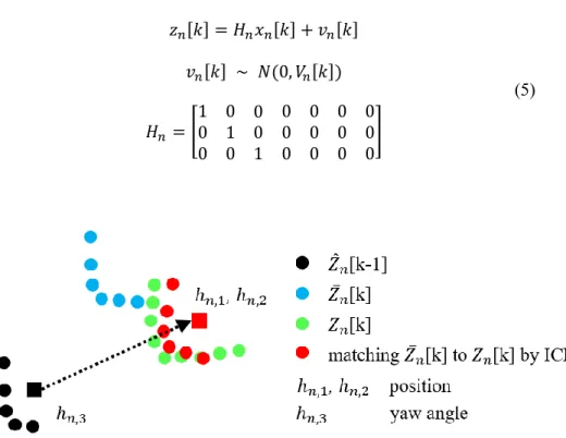
EKF is applied for measurement update of clusters. In the proposed approach, the three measurements obtained from 𝑍_𝑛 are the position and yaw angle of the moving objects. In formula (5), measurement for the EKF is 𝑧_𝑛 that is expressed as 3D vector and each element of 𝑧𝑛 represents the position of mean point and yaw angle of the moving object at 𝑋_𝐿𝑌_𝐿, respectively. The position measurement of n-th track is considered as the mean of the matched 𝑍̅𝑛, after matching 𝑍̅𝑛 to 𝑍𝑛 by ICP algorithm. The moving direction of the object is the direction of the displacement vector from the mean of 𝑍̂_𝑛[𝑘 − 1]

to the mean of matched 𝑍̅_𝑛[k]. This process is visualized in figure 6, and the measurement model using these measurements is composed of a linear model as shown in (5), assuming that the measured values have white Gaussian noise with covariance matrix of 𝑉_𝑛.

(32)

22

𝑧𝑛[𝑘] = 𝐻_𝑛𝑥𝑛[𝑘] + 𝑣_𝑛[𝑘]

𝑣_𝑛[𝑘] ~ 𝑁(0, 𝑉_𝑛[𝑘])

𝐻_𝑛= [ 1 0 0

0 1 0

0 0 1

0 0 0

0 0 0 ]

(5)

Fig. 6 The measurement of n-th track from corresponding cluster and its matching process.

(33)

Chapter 5. Experimental Results

23

Chapter 5

Experimental Results

The only difference of existing GMFT and proposed approach is whether or not it is fused and interacted with mapping method. Considering the error of state estimation, code operation time, detection rate and fail cases are important, the proposed approach is verified by comparing with the case where GMFT is used alone.

(34)

24

5.1 Vehicles and sensors configuration

Driving data is obtained at the Nambu-Beltway using IONIQ and K5, which play a role as ego(hunter) vehicle and target vehicle, respectively. The hunter, IONIQ has 6 IBEO 2D LiDAR sensor. To compare the performance of proposed perception algorithm and existing GMFT algorithm, it is necessary to collect reference data of the target. Thus, two vehicles are equipped with RT- GPS for precise localization and RT-Range for time sync of these two RT-GPS.

Vehicles and sensors configuration are summarized in figure 5, 7, 8. All communication, algorithm, and computation are operated on Matlab-Labview environment with Intel Core i7-4790 4.00GHz CPU.

(35)

25 Fig. 7 Sensor configuration.

(36)

26 Fig. 8 FOV and detection limit of LiDAR

(37)

27

5.2 Detection rate of moving object

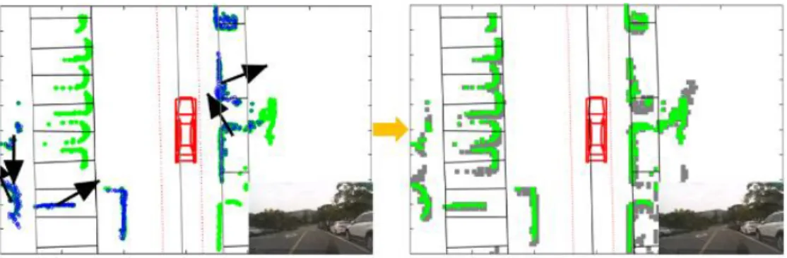
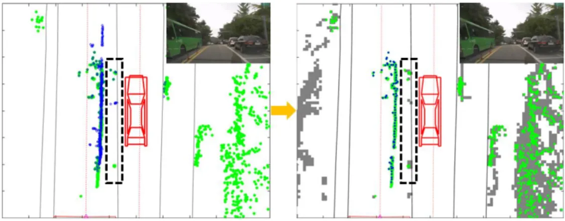
Figure 9, 10 shows representative detection fail case of GMFT and its improvement by proposed approach. In figure 10 where the stationary vehicle Fig. 10 Improvement of fail case – Median separator

Fig. 9 Improvement of fail case – Parking lot

(38)

28

on the right side, the median separator on the left side, and the moving vehicle is located in the vicinity, conventional GMFT fails to classify the LiDAR points into true clusters and to detect them by tying the wrong points together. On the other hand, since the proposed approach transmits predicted obstacle information before the DATMO module is activated, it excludes them in advance and starts clustering, which shows much better detection results.

Figure 9 shows a parking lot with many stopped vehicles. All vehicles are about 20cm apart and it is very difficult for GMFT algorithm to classify them into different clusters and conclude that they are not moving vehicles. This error comes from a variety of factors, such as clustering error since each vehicle is too close with each other. Moreover, points that start from a certain time in a blind spot may look like a moving vehicle. The proposed approach resolves this problem successfully. Since the proposed method stores probability values for every grid, it judges that it is a stop point based on the Bayesian rule even if there are sudden arising points from the blind spot. Thus, obviously, DATMO gets to knows that these vehicles are not moving vehicles, so it can easily detect the vehicles that are really moving around.

Beyond this simple example, a full evaluation of the detection rate is shown in figure 11. In a complex urban road, all the vehicles inside the surrounding ROI are checked by manual operation. After both the proposed approach and the existing approach are performed, the detection results are

(39)

29

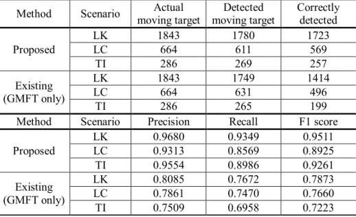
recorded as shown in the figure. All of the above steps are conducted at every frame and summed up. Total results for all frames with respect to each driving scenario are summarized in the top of table 1. Furthermore, these are recalculated to performance indicator, Precision, Recall, and F1 score.

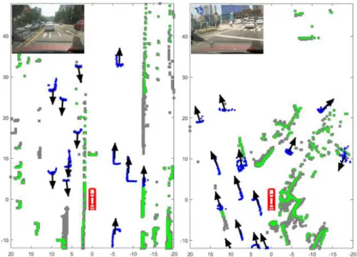
Fig. 11 Evaluation of detection rate with complex traffic, at Nambu-Beltway.

Actual moving targets are labeled by manually, and black arrows are detected moving target through proposed approach. Blue means cluster of tracks, green is LiDAR point cloud, gray is SOM.

(40)

30

Table 1 Detection result of moving vehicles and evaluation by three performance indicators

Performance indicators are expressed at the bottom of table 1. Precision is the ratio of correctly predicted value to the total predicted value (correctly detected/detected), Recall is the ratio of correctly predicted value to the all value in actual class (correctly detected/actual), and F1 Score is the weighted average of Precision and Recall (2*Recall * Precision / (Recall + Precision)).

All indicators are improved by 15~30% for all scenarios. An increase of Precision means that the number of false alarm has decreased, and larger Recall means that the frequency of false negative has been reduced.

Method Scenario Actual moving target

Detected moving target

Correctly detected Proposed

LK 1843 1780 1723

LC 664 611 569

TI 286 269 257

Existing (GMFT only)

LK 1843 1749 1414

LC 664 631 496

TI 286 265 199

Method Scenario Precision Recall F1 score

Proposed

LK 0.9680 0.9349 0.9511

LC 0.9313 0.8569 0.8925

TI 0.9554 0.8986 0.9261

LK 0.8085 0.7672 0.7873

LC 0.7861 0.7470 0.7660

TI 0.7509 0.6958 0.7223

(41)

31

5.3 State estimation accuracy of moving object

In this section, estimated position, velocity, and yaw angle of target vehicle are validated using reference data from RT-range for 3 different scenarios, Lane Keeping(LK), Lane Change(LC), and Turning at the Intersection(TI), respectively. Driving data had to be collected considering that the main contribution of this study is to distribute mapping function to separated module (SOM). Thus, all scenarios selected to include both moving vehicles and static obstacle such as pole, curb, stopped vehicles. Each scenario is conducted 10 times and the speed is controlled within 50kph due to the traffic condition of Nambu-Beltway.

Histogram of error distribution is indicated in figure 12 with respect to each scenario. Blue and red denote proposed DATMO + Mapping (GMFT + SOM) approach and conventional DATMO (GMFT) only, respectively. As shown in the histogram, some bias exists due to the fact that the mounting position of GPS antenna does not coincide with the center of the vehicle and unique characteristic of RT-range by calibration. Thus, the standard deviation is valid as the main indicator to evaluate the estimation accuracy.

(42)

32

Fig. 12 Error distribution of position, velocity, and yaw angle with respect to 3 driving scenarios, Lane keeping(LK), Lane changing(LC), and Turning at intersection(TI).

(43)

33

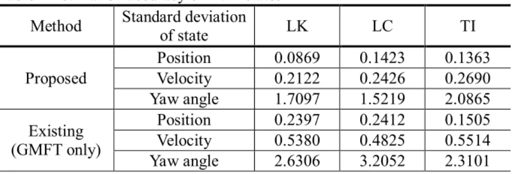
GMFT+SOM shows better standard deviation as shown in table 2. For all scenarios and all states, the standard deviation is larger for the case of the existing method than the proposed algorithm. Especially, in the case of figure 12-(c), (f), the significant mean error of yaw angle occurs in the existing method.

This is because the median strip that exists at the left side of target vehicle disturbs clustering. In accordance with the intention of this study, the proposed algorithm help clustering to avoids from being disturbed by peripheral static obstacles, thus indicating less mean error and less standard deviation.

Table 2 Estimation accuracy of main states

In general, due to the limit of 2D LiDAR itself, point cloud of static obstacle can be observed like a moving object even though the points are of a static object. In some case, as the moving vehicle moves past, the part of static obstacle that was blind begins to be observed, thus it can be seen as a moving object in the existing method. This is because the GMFT judges whether or not it is moving based on the flow of points. However, the proposed algorithm can

Method Standard deviation

of state LK LC TI

Proposed

Position 0.0869 0.1423 0.1363 Velocity 0.2122 0.2426 0.2690 Yaw angle 1.7097 1.5219 2.0865 Existing

(GMFT only)

Position 0.2397 0.2412 0.1505 Velocity 0.5380 0.4825 0.5514 Yaw angle 2.6306 3.2052 2.3101

(44)

34

be free from this problem because the SOM maintains the probability of static obstacle for all grid in advance, thus GMFT can eliminate unnecessary points before clustering. It is reasonable that this leads to improvements in state estimation accuracy of moving vehicles.

5.4 Code operation time

Algorithms are run on the platform described in 5.1. Code operation time is recorded at every time step and the results for two approaches are summarized in table 3, which includes all scenario LK, LC, and TI. While the existing method is operated with GMFT only, results of the proposed approach are separated into sub-function in order. The proposed approach consumes a certain amount of time in the sub-function. However, in the GMFT process of the proposed approach, time is dramatically reduced enough to offset the loss in the other sub-functions. This result accurately confirms the intention of the interaction between DATMO and SOM, which distributing the roles performed by DATMO (GMFT) in the existing research, thereby reducing the calculation burden. As a result, the total elapsed time for the whole perception algorithm is greatly reduced. This also satisfies to maintain operation time less than 80 msec, which corresponds to the operation frequency of IBEO LiDAR, 12.5Hz.

(45)

35 Table 3 Code operation time of sub-function

Method Time (ms)

SOM GMFT SOM

Total (ms) Predict Clustering Track

management Update

Proposed Mean 8.1 5.7 24.8 6.2 44.8

Max 13.2 15.9 75.5 8.5 113.1

Mean – 13.7 86.4 – 100.1

Max – 31.5 125.7 – 157.2

(46)

Chapter 6. Conclusion and Future Work

36

Chapter 6

Conclusion and Future Work

6.1 Conclusion

In this paper, a novel fusion approach based on the interaction between Static Obstacle Map (SOM) method and Geometric Model-Free Tracking (GMFT) algorithm is presented to improve detection and tracking performance for real-time, urban autonomous driving. Interaction concept is designed to divide the role of the construction of a map that consists of static objects only

(47)

37

and the role of tracking of moving objects such as moving vehicles. Detection rate of moving objects, state estimation accuracy of target, and calculation burden have shown problems under the existing approach, which is a conventional method using only DATMO algorithm, and much of them are solved by the proposed approach.

The main contribution of this study is distributing roles of algorithms according to the motion state of the LiDAR point cloud. Thus, advantages of the proposed approach are more evident in complicated driving situation include moving objects and static obstacles include poles, cones, curbs, sidewalks, stop vehicles and all geographic features. The comparative advantage of the proposed method may be relatively small in an uncrowded road situation, but under such circumstances, the existing method also shows good performance and is less likely to cause problems.

6.2 Future works

The GMFT algorithm, which is selected for achieving DATMO, assumes that the shape of consecutive LiDAR point does not change dramatically.

However, in real driving circumstances, above assumption does not match due to FOV (Field of View) of LiDAR, blind spot by any objects, or in case of

(48)

38

moving vehicle passes ego vehicle by very high speed. Therefore, Geometric Model-Based Tracking (GMBT) or feature-based matching approach need to be dealt with in future work.

In addition, shape extraction is helpful if it is added to this study. Due to the geometric relationship, the center of vehicles is varied according to whether the classified clusters consist of only one side of vehicles, or it includes both side and the back side of vehicles. This would improve estimation accuracy of position and yaw angle than this study.

(49)

Bibliography

39

Bibliography

[1] Wang, Chieh-Chih, et al. "Simultaneous localization, mapping and moving object tracking." The International Journal of Robotics Research 26.9 (2007): 889-916.

[2] Moosmann, Frank, and Christoph Stiller. "Joint self-localization and tracking of generic objects in 3D range data." 2013 IEEE International Conference on Robotics and Automation. IEEE, 2013.

[3] Siew, Peng Mun, Richard Linares, and Vibhor Bageshwar.

"Simultaneous Localization and Mapping with Moving Object Tracking in 3D Range Data using Probability Hypothesis Density (PHD) Filter." 2018 AIAA Information Systems-AIAA Infotech@

Aerospace. 2018. 0507.

[4] Lidoris, Georgios, Dirk Wollherr, and Martin Buss. "Bayesian state

(50)

Bibliography

40

estimation and behavior selection for autonomous robotic exploration in dynamic environments." 2008 IEEE/RSJ International Conference on Intelligent Robots and Systems. IEEE, 2008.

[5] Vu, Trung-Dung, Julien Burlet, and Olivier Aycard. "Grid-based localization and local mapping with moving object detection and tracking." Information Fusion 12.1 (2011): 58-69.

[6] Wolf, Denis, and Gaurav S. Sukhatme. "Online simultaneous localization and mapping in dynamic environments." IEEE International Conference on Robotics and Automation, 2004.

Proceedings. ICRA'04. 2004. Vol. 2. IEEE, 2004.

[7] Pancham, Ardhisha, Nkgatho Tlale, and Glen Bright. "Literature review of SLAM and DATMO." (2011).

[8] Kim, B., Yi, K., Yoo, H. J., Chong, H. J., & Ko, B. (2014). An IMM/EKF approach for enhanced multitarget state estimation for application to integrated risk management system. IEEE Transactions on Vehicular Technology, 64(3), 876-889.

[9] Thrun, Sebastian, Wolfram Burgard, and Dieter Fox. Probabilistic robotics. MIT press, 2005.

[10] Wang, Chieh-Chih, et al. "Simultaneous localization, mapping and moving object tracking." The International Journal of Robotics Research 26.9 (2007): 889-916.

(51)

Bibliography

41

[11] Bouzouraa, Mohamed Essayed, and Ulrich Hofmann. "Fusion of occupancy grid mapping and model based object tracking for driver assistance systems using laser and radar sensors." 2010 IEEE Intelligent Vehicles Symposium. IEEE, 2010.

[12] Saval-Calvo, Marcelo, et al. "A review of the Bayesian occupancy filter." Sensors 17.2 (2017): 344.

[13] Sualeh, Muhammad, and Gon-Woo Kim. "Dynamic Multi-LiDAR Based Multiple Object Detection and Tracking." Sensors 19.6 (2019):

1474.

[14] Na, Kiin, et al. "RoadPlot-DATMO: Moving object tracking and track fusion system using multiple sensors." 2015 International Conference on Connected Vehicles and Expo (ICCVE). IEEE, 2015.

[15] Magnier, Valentin, Dominique Gruyer, and Jerome Godelle.

"Automotive LIDAR objects detection and classification algorithm using the belief theory." 2017 IEEE Intelligent Vehicles Symposium (IV). IEEE, 2017.

[16] Zhang, Liang, et al. "Multiple vehicle-like target tracking based on the velodyne lidar." IFAC Proceedings Volumes 46.10 (2013): 126-131.

[17] Hwang, Soonmin, et al. "Fast multiple objects detection and tracking fusing color camera and 3D LIDAR for intelligent vehicles." 2016 13th International Conference on Ubiquitous Robots and Ambient

(52)

Bibliography

42 Intelligence (URAI). IEEE, 2016.

[18] Vaquero, Victor, Ely Repiso, and Alberto Sanfeliu. "Robust and real- time detection and tracking of moving objects with minimum 2D LIDAR information to advance autonomous cargo handling in ports." Sensors 19.1 (2019): 107.

[19] Asvadi, Alireza, et al. "3D Lidar-based static and moving obstacle detection in driving environments: An approach based on voxels and multi-region ground planes." Robotics and Autonomous Systems 83 (2016): 299-311.

[20] Llamazares, Ángel, Eduardo J. Molinos, and Manuel Ocaña.

"Detection and Tracking of Moving Obstacles (DATMO): A Review." Robotica: 1-14.

(53)

초 록

43

초 록

자율주행을 위한 정지 장애물 맵과 GMFT 융합 기반 이동 물체 탐지 및 추적

라이다 센서의 측정 정밀성을 기반으로 하여 DATMO, 즉 이동 물체 탐지 및 추적은 자율주행 인지 분야의 매우 중요한 주제로 발 전되어 왔다. 그러나 다양한 종류의 차량에 의해 도로 상황이 복잡 한 점 및 도로 특유의 복잡한 지형적 특성 때문에 클러스터링

(Clustering)의 실패 사례가 종종 발생할 뿐만 아니라 인지 알고리즘

의 계산 부담도 증가한다. 이러한 문제를 극복하기 위해 이 논문에 서는 DATMO 알고리즘과 맵핑 알고리즘을 통합하여 새로운 접근법 을 제시하였다. DATMO 와 맵핑 알고리즘은 각각 이동 물체와 정지 물체의 상태를 추정하는데에 특화되어있기 때문에 두 알고리즘은 서로의 출력을 입력으로 사용하여 추정 성능을 향상시킬 수 있다.

전체 인지 알고리즘은 DATMO 와 맵핑 알고리즘을 포함하는 피드백 루프 구조로 재구성된다. 또한 두 알고리즘은 각각 Geometric Model- Free Tracking(GMFT)과 베이지안 룰 기반의 혁신적인 Static Obstacle

(54)

초 록

44

Map(SOM)으로 수정되어 서로의 출력을 필터링 프로세스의 측정값

으로 사용한다. 이 연구에서 제시한 통합 인지 알고리즘은 RTK DGPS와 RT Range 장비, 그리고 2차원 LiDAR 를 장착한 차량을 이 용하여 수집한 데이터를 통해 성능을 평가하였다. 기존의 DATMO 연구에서 발생했던 몇 가지 일반적인 클러스터링 실패 사례가 감소 하였고 전체 통합 인지 과정에 대한 알고리즘 작동 시간이 감소함 을 확인하였다. 특히, 이동하는 물체의 위치, 속도, 방향을 추정한 결과는 RT Range 장비로 측정한 실제 값과 기존 방식 대비 더욱 적 은 오차를 보여주었다.

주요어: 라이다, 맵핑, 정지 장애물 맵, 이동 물체 탐지 및 추적, Geometric Model-Free Tracking, 베이지안 룰