저작자표시-비영리-변경금지 2.0 대한민국 이용자는 ... - S-Space

(1)

저작자표시-비영리-변경금지 2.0 대한민국 이용자는 아래의 조건을 따르는 경우에 한하여 자유롭게

l 이 저작물을 복제, 배포, 전송, 전시, 공연 및 방송할 수 있습니다. 다음과 같은 조건을 따라야 합니다:

l 귀하는, 이 저작물의 재이용이나 배포의 경우, 이 저작물에 적용된 이용허락조건 을 명확하게 나타내어야 합니다.

저작권법에 따른 이용자의 권리는 위의 내용에 의하여 영향을 받지 않습니다. 이것은 이용허락규약(Legal Code)을 이해하기 쉽게 요약한 것입니다.

Disclaimer

저작자표시. 귀하는 원저작자를 표시하여야 합니다.

비영리. 귀하는 이 저작물을 영리 목적으로 이용할 수 없습니다.

변경금지. 귀하는 이 저작물을 개작, 변형 또는 가공할 수 없습니다.

(2)

이학석사 학위논문

SF Network

Squeezed Fusion Network using Fully Convolutional Network for Biomedical

Image Segmentation

생체 이미지 분할을 위한 완전 합성곱 신경망을 이용한 SF 네트워크

2019년 8월

서울대학교 대학원

협동과정 계산과학전공

김 종 태

(3)

SF Network

Image Segmentation

생체 이미지 분할을 위한 완전 합 성곱 신경망을 이용한 SF 네트워크

지도교수 강 명 주

이 논문을 이학석사 학위논문으로 제출함

2019년 4월

서울대학교 대학원

협동과정 계산과학전공

김 종 태

김 종 태의 이학석사 학위논문을 인준함

2019년 5월

위 원 장

(인)

부 위 원 장

(인)

(4)

SF Network

Image Segmentation

by

Jongtae Kim

A DISSERTATION

Submitted to the faculty of the Graduate School in partial fulfillment of the requirements

for the degree of Master of Science in the Department of

Computational Science and Technology Seoul National University

August 2019

(5)

(6)

Abstract

In recent years, with the development of deep learning technology, complex computation and large-scale image processing have become possible. Such image processing techniques are widely applied in research fields such as Aerospace, Autonomous Driving, Biotech, and semiconductor engineering.

Since medical image processing is so complicated, the deep learning method is particularly useful for extracting and dividing the boundaries of electron microscope (EM) images. For this reason, U-Net was proposed to achieve more accurate results, and then FusionNet was proposed. However, as the deep learning networks have developed, there has been the problem that re- quires more and more parameters for this kind of learning.

In this paper, we introduce SF network, a new deep neural network architecture for automatic image segmentation with fewer parameters than existing deep learning methods. In order to avoid increasing the size of the feature map as the network depth increases, 1×1 convolution was added to improve the performance by reducing the number of parameters and applying a skip connection.

The performance of the proposed image segmentation method is demon- strated by comparing its performance with that of previous architectures from the ISBI 2012 EM segmentation data and Mouse Piriform Cortex EM segmentation data. By using V_score^rand andV_score^dice to calculate the metric similarity to a ground truth image, the proposed model had slightly better results, compared with previous methods in reference to metrics.

Key words: Deep Learning, Image segmentation, fully convolutional network, U-Net, FusionNet

Student Number: 2017-22461

(7)

Image segmentation is one of the core computer vision technologies needed to understand the visual environment completely, which is a problem of classification into several predefined classes in pixels. Semantic image segmentation is used in a variety of applications including autonomous navigation, semantic 3D reconstruction of indoor and outdoor areas, medical image analysis, and virtual and augmented reality systems [1].

Previous semantic image segmentation studies have attempted to solve problems through classifier methods such as SVM using human-designed key points such as SIFT, HoG, and SURF [2, 3]. In recent years, instead of the key points and classification schemes devised by humans, deep convolutional neural network (DCNN) research has been actively used to extract data-based key points and to classify using large-scale learning data. The DCNN has been applied to various computer vision problems and research and performed better than the existing techniques actively being carried out [4].

Particularly, artificial intelligence has made remarkable progress in solv- ing problems involving very complex decision-making, comparable to human capabilities. The convolutional neural network (CNN) model, which is often used in a deep neural network called deep learning, is able to extract hier- archical image features from input data, so it showed excellent performance for visual recognition problems such as image segmentation. Performance im- provements of these algorithms were mainly based on the development of a high-performance parallel computing technology using GPU and the develop-

(9)

ment of an artificial neural network learning algorithm using back propaga- tion. In addition, a large-scale image database collected by computer vision researchers is used as important materials for learning and performance mea- surement [5].

Such an artificial intelligence technology has recently been used for image segmentation in medical imaging using electron microscopy (EM) data [6, 7, 8]. The reason why artificial intelligence technology is suitable for this study can be explained as follows. First of all, the data accumulated from many experiences are increasing, and using this data, we can obtain better outputs than existing modeling-based image segmentation algorithms. For a problem requiring a decision, in particular, performance comparable to human accuracy is derived through recent deep learning results, and it can be used in automation data analysis processes that currently require a great deal of manual work. Pixel-wise classification using a fully connected layer has been used for image segmentation [9], when performing image segmentation with existing deep learning. However, when this method is used, there are drawbacks: the loss of geometric properties in the input image and the requirement for a huge amount of computation.

Therefore, to overcome these drawbacks, J. Long et al [4] proposed a fully convolutional network (FCN). The deep learning method that performed successfully for image segmentation of EM data using this FCN is more developed in U-Net [7], which was proposed by Ronneberger et al in 2015. U-Net included an image segmentation method with simple structures using such as convolution, deconvolution, maxpooling, and skip connection. Through this method, image segmentation was successfully performed. Using the existing deep learning method, U-Net was manifested as a standard model with state- of-the-art capabilities. However, U-Net has the following drawbacks. First, the number of feature maps increases significantly due to concatenation. Sec- ond, as the number of layers increases, the number of convolution parameters required for learning also increases. Based on U-Net, The FusionNet which was proposed by Quan et al. [8] provides more advanced results. Overall, it has an architecture similar to that of U-Net, but has the following two signif- icant differences.

(10)

1. By adding residual blocks, it can extract well the high level features of CNN.

2. In the skip connection, concatenation is used in U-Net, whereas in Fu- sionNet, a summation-based skip connection is applied to maintain the characteristics of the previous CNN.

Particularly, as mentioned difference above 1, With some residual blocks, we can see that the whole network is deeper than U-Net. However, when adding such residual blocks, the number of parameters increases more rapidly than in the case of U-Net. As such, there is still the drawback of requiring more memory and learning time for the GPU to be involved. Therefore, in this paper, we propose a network that is similar to the existing method but yields somewhat better results while reducing the number of learning parameters of the existing network to a much smaller number. The proposed deep learning network is similar to that of FusionNet, but the number of feature maps used in the convolution layer after residual block is fixed at 64; then reduced to 32 by 1×1 convolution. After that, differently from FusionNet, feature maps are constructed using concatenation with the skip connection of previous same size’s convolution block. Using this method, we confirm that the method proposed in this paper obtains better results than with the previous U-Net and FusionNet using ISBI 2012 data and Mouse Piriform Cortex data evaluation.

This paper is organized as follows. In Section 2, we give a brief introduction to U-Net and FusionNet, which provide the bases for this paper. In Section 3, we describe an image segmentation network using a small number of parameters for the learning proposed in this paper. The validation of this network is verified through experiments using the ISBI 2012 EM segmentation data and Mouse Piriform Cortex EM segmentation data in Section 4. Finally, the conclusions are presented in Section 5.

(11)

Chapter 2

Related work

FusionNet: FusionNet was proposed by Quan et al. in 2016. The network is for performing semantic segmentation and is based on the U-Net proposed in 2015. U-Net performs image segmentation using FCN, which concatenates feature maps of previously obtained convolution blocks in deconvolution layers and obtains simple but powerful results. Since the FCN does not use a fully connected layer, it has the advantage of preserving geometric data on the image.

In FusionNet, higher level features can be extracted using residual blocks.

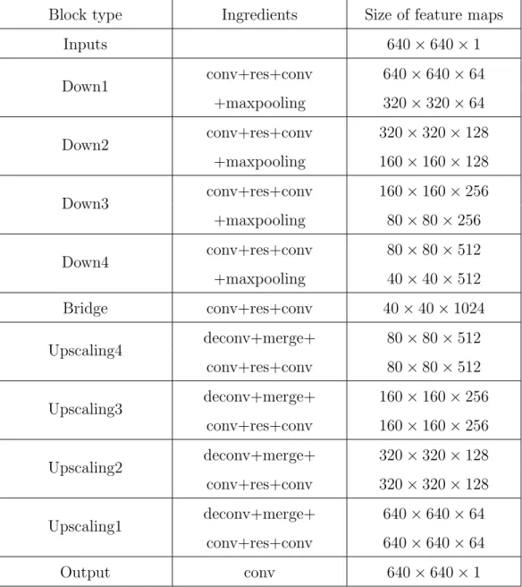
Then, the feature value becomes stronger by adding the previous convolution feature maps and the deconvolution feature maps. The entire network is constructed symmetrically by this process. Table 2.1 shows that FusionNet is a symmetric structure centering on the bridge part. Based on the FCN method, FusionNet used the ISBI 2012 EM segmentation challenge data [8] to achieve the best results compared with the existing segmentation algorithms, including U-Net.

However, when such a method is used, it can be seen that the number of learning parameters increases rapidly. The number of learning parameters is 25M for U-Net and 69M for FusionNet. Therefore, the following sections describe the networks that provide better results while reducing the number of learning parameters.

(12)

Block type Ingredients Size of feature maps

Inputs 640×640×1

Down1 conv+res+conv 640×640×64

+maxpooling 320×320×64

Bridge conv+res+conv 40×40×1024

Upscaling4 deconv+merge+ 80×80×512

conv+res+conv 80×80×512

Output conv 640×640×1

Table 2.1: Summary of FusionNet

(13)

Chapter 3

Description of SF Network Architecture

3.1 Explains for SF Network

In this section, our proposed SF Network is described. In the case of FusionNet and U-Net described above, FCN was applied. Therefore, in this paper, image segmentation is also performed using FCN as in the previous method.

In SF Network, as with FusionNet, the size of both the input and output image was fixed at 640×640×1. In the downscaling operation, there are blocks having the following structure. First, there is a 3×3 convolution layer. The depth size of the feature map is set to 64 while passing through this layer. The result is used as two inputs at the next stage. One input passes to the output through three convolution layers, and the other passes through the short skip connection to the output. And then we add the two outputs. This is called the residual block. After this passes through the 3×3 convolution layer again, the number of feature maps is adjusted to 32 using 1×1 convolution. After 1×1 convolution, the result is used as two inputs. One is maxpooling, and the other is concatenation after the deconvolution work. In this network, we always perform batch normalization and ReLU after the convolutions.

In the upscaling operation, the deconvolution layer is used to increase the length to two times the width and height while maintaining the number of

(14)

the same size feature map created by downscaling. Then, as done previously, the concatenated layer passes 3×3 convolution, residual block, 3×3 convolution, and 1×1 convolution. See Figure 3.1 for more details.

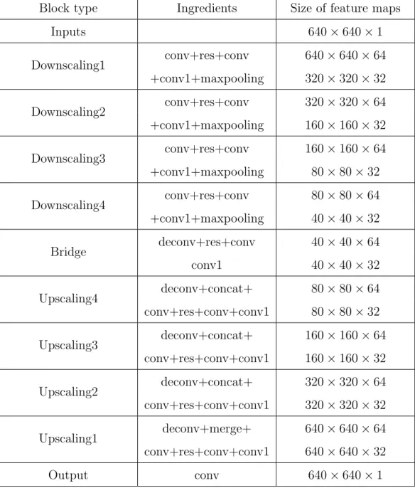
Therefore, when using such structures, it can be seen that, except for the input/output image, the number of feature maps is always 64 before the 1×1 convolution and then remains constant at 32 thereafter. For more specific networks, see Table 3.1 below. Here, conv1 means 1×1 convolution and concat means concatenation.

3.2 Comparison with Other Networks

Same Compared to U-Net, SF Network has a larger input/output image size and a much deeper network. Compared to FusionNet, SF Network has a very similar structure, but there are two differences. First, it is possible to reduce the feature map depth by taking a 1×1 convolution after the 3×3 convolution behind the residual block. Second, after deconvolution as done in U-Net in the upscaling step, we use concatenation instead of summation in the skip connection.

By using these methods, we constructed our network with far fewer parameters than U-Net and FusionNet (U-Net: 25M, FusionNet: 69M). In particular, for U-Net, both input and output image sizes are small compared to those of SF Network, but the number of parameters for learning is larger.

However, in the case of SF Network, the network was constructed using only 1.6M parameters.

(15)

640×640 Ouputimage 640×640Inputimage

320×320

160×160

80×8040×40

3×3 convolutionResidual block : (3×3 conv)×3+skip connection1×1 convolutionMaxpoolingdeconvolution +

(16)

Block type Ingredients Size of feature maps

Inputs 640×640×1

Downscaling1 conv+res+conv 640×640×64 +conv1+maxpooling 320×320×32 Downscaling2 conv+res+conv 320×320×64 +conv1+maxpooling 160×160×32 Downscaling3 conv+res+conv 160×160×64 +conv1+maxpooling 80×80×32

Downscaling4 conv+res+conv 80×80×64

+conv1+maxpooling 40×40×32

Bridge deconv+res+conv 40×40×64

conv1 40×40×32

Upscaling4 deconv+concat+ 80×80×64

conv+res+conv+conv1 80×80×32 Upscaling3 deconv+concat+ 160×160×64

conv+res+conv+conv1 160×160×32 Upscaling2 deconv+concat+ 320×320×64 conv+res+conv+conv1 320×320×32

conv+res+conv+conv1 640×640×32

Output conv 640×640×1

Table 3.1: Summary of SF Network

(17)

Chapter 4

Experimental Result

4.1 Experiment Settings

In this section we describe how our proposed architecture was verified ex- perimentally. The experimental environment was an Intel Core i5-6500 3.20 Hz, 16 GB RAM, and a Tesla K80 GPU. The algorithm implementation used Python and TensorFlow. The loss function used in the training was the Mean Square Error (MSE) and the optimizer used Adam. The learning rate was set to 0.0001, the epoch was set to 300, and the batch size was set to 2.

4.2 Experiment Evaluation

In this paper, we used two metrics for verification of the similarity between the GT (ground truth) image and the prediction result: V_score^rand and V_score^dice [10, 11]. The V_score^rand calculation was performed using script ImageJ [12]. The experimental data used for the verification included the EM data [10] in the two-dimensional electron microscopy segmentation challenge of ISBI 2012, and the Mouse Piriform Cortex EM data [13] disclosed to the public.

To evaluate the performance of our method, we follow theV_score^randmentioned in [10] on the two EM segmentation tasks. Suppose that S is the predicted segmentation result andT is the ground truth. We define a p_ij as the probability of a randomly selected pixel belongs to the i-th segment in S and the

(18)

as follows:

V_split^rand = P

ijp_ij² P

kt_k² V_merge^rand =

P

ijp_ij² P

ks_k² wheres_i =P

jp_ij andt_i =P

ip_ij.V_split^rand score andV_merge^rand score are defined as the probability of two randomly selected voxels are from the same segment in S when given they belong to the same segment in T and the probability of two randomly selected voxels are from the same segment in Twhen given they belong to the same segment inSrespectively. TheV_split^randscore andV_merge^rand score become higher when there are less split and merge errors respectively.

In order to combine the two scores together, the weighted harmonic mean is used:

V_α^rand =

P

ijpij2

αP

ks_k²+ (1−α)P

kt_k²

The highest value obtained by changing the α value from 0.1 to 1.0 in increments of 0.1 is referred to as the V_score^rand value.

The evaluation of our experiment is based on a script in ImageJ [12], which calculates the best V_score^rand after thinning over threshold in different values for the probability map.¹

The Dice coefficient [14] (V_score^dice), also called the overlap index, is the most used metric in validating medical volume segmentations. In addition to the direct comparison between automatic and ground truth segmentations, it is common to use the V_score^dice to measure reproducibility (or repeatability). Zou et al. [15] used the V_score^dice as a measure of the reproducibility as a statistical validation of manual annotation where segmenters repeatedly annotated the same MRI image, then the pair-wise overlap of the repeated segmentations is calculated using the V_score^dice, which is defined by

1http://imagej.net/Segmentation evaluation after border thinning Script

(19)

V_score^dice = 2|s_g∩s_t|

|s_g|+|s_t|= 2T P

2T P +F P +F N

The Jaccard index (JAC) [16] between two sets is defined as the intersec- tion between them divided by their union, that is

J AC = |sg∩st|

|s_g∪s_t|= T P

P T +F P +F N

We note that JAC is always larger than DICE except at the extrema 0, 1 where they are equal. Furthermore, the two metrics are related according to

J AC = |s_g ∩s_t|

|s_g ∪s_t|= 2|s_g∩s_t|

2(|s_g|+|s_t| − |s_g∩s_t|)= V_score^dice 2−V_score^dice Similarly, one can show that

V_score^dice = 2J AC 1 +J AC

That means that both of the metrics measure the same aspects and provide the same system ranking.

4.3 Result Comparison

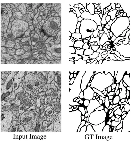
The ISBI 2012 EM data consists of an input image and a ground truth image, the data has a total of 30 sections. The ground truth image consists of white pixels, with black pixels that form the boundary. Mouse Piriform Cortex EM data consists of four stacks, each consisting of 168, 170, 169, and 121 images. The sizes of the images are 255×255, 512×512, 512×512, and 256×256, respectively. Because of the structure of SF Network, the input size is 640×640×1, so the image data should be resized and used at the input image size. In this paper, in order to minimize image data distortion dur-

(20)

stack3, which were similar to the input image size. Image examples from the ISBI 2012 EM data and Mouse Piriform Cortex EM are shown in Figure 4.1

GT Image Input Image

Figure 4.1: Example for dataset: Left is the ISBI 2012 EM (stack 1/30) and right is the Mouse Piriform Cortex EM dataset (stack2 1/170)

In the ISBI 2012 data, 80% of the images were used for training and 20%

of the images were used for verification (1-24 for training / 25-30 for testing).

In the Mouse Piriform cortex data, we used stack2 and 60% images of stack3 for training, and 40% of the stack3 images for verification (stack2 and stack3 1-100 for training / stack3 101-169 for testing).

(21)

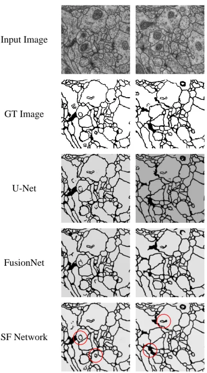
The experimental results obtained using the data are as follows. First, experiments were performed using the ISBI 2012 EM data. As with U-Net and FusionNet previously used, the ISBI 2012 data was subjected to data augmentation to obtain more image data. The number of data was increased by eight times using the method of rotating the original image data and the method of mirroring the original image [8].

As can be seen from the results in Figure 4.2, the image segmentation results are generally similar. Especially when compared with U-Net and Fu- sionNet, the red circle part shows that SF Network is more similar to the GT image.

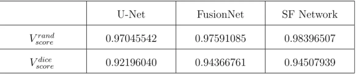
The results of V_score^rand and V_score^dice are shown in Table 4.1. Looking at the results of U-Net and FusionNet used as a comparison group, we can see that the results are generally similar, but the results of SF Network are slightly better.

U-Net FusionNet SF Network

V_score^rand 0.97045542 0.97591085 0.98396507

V_score^dice 0.92196040 0.94366761 0.94507939

Table 4.1: Evaluation of ISBI 2012 EM dataset

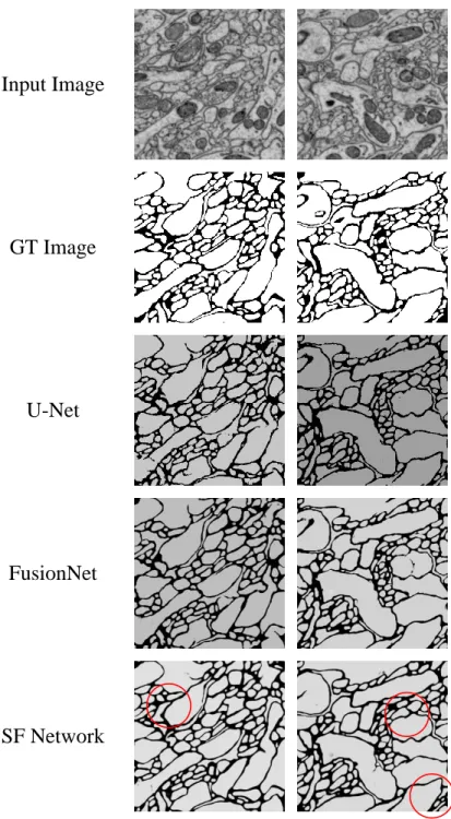
Next, the results obtained using the Mouse Piriform Cortex dataset were confirmed. In this case, the number of data was sufficient, so we did not need to execute data augmentation work. As in the previous case, the visualized result of image segmentation was almost the same as the previous result in Figure 4.3. In the image of the SF Network, the red circle indicates that the SF Network output is more similar to the GT image than were those of U-Net and FusionNet.

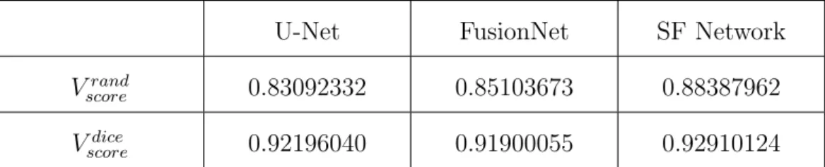
The results of V_score^rand and V_score^dice are shown in Table 4.2. As before, the results are comparable with those of U-Net and FusionNet overall, but the results of SF Network are slightly better.

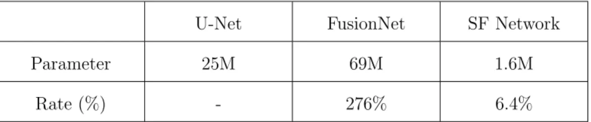
Finally, we compared the number of parameters applied to each network.

(22)

V_score^rand 0.83092332 0.85103673 0.88387962

V_score^dice 0.92196040 0.91900055 0.92910124

Table 4.2: Evaluation of Mouse Piriform Cortex dataset

million parameters in FusionNet. However, the proposed SF Network in this paper applied only 1.6 million parameters.

We confirmed that it is possible to obtain results very similar to existing results (but slightly better) using only about 6.7% of the parameters used by the U-Net and 2.33% used by the FusionNet model.

Parameter 25M 69M 1.6M

Rate (%) - 276% 6.4%

Table 4.3: Parameter comparison

(23)

Input Image

GT Image

U-Net

FusionNet

SF Network

Figure 4.2: Original, ground truth, and experimental result image in the ISBI

(24)

Input Image

GT Image

U-Net

FusionNet

SF Network

Figure 4.3: Original, ground truth, and experimental result image in the Mouse Piriform cortex EM dataset

(25)

Chapter 5 Conclusion

In this paper, we introduced a deep learning network called SF Network that is much more lightweight than the existing networks. Through the FCN already used in semantic segmentation by the deep learning method, the parameters for learning with SF Network is less than 3% that of FusionNet and less than 7% that of U-Net. However, the results are very similar, but slightly better.

This shows that a deep learning model with a small size network for semantic segmentation can also get good results. The results of this paper are expected to be developed into a lightweight model, deep running architecture and commercialized in environments such as mobile devices.

(26)

Bibliography

[1] Md Amirul Islam, Neil Bruce, and Yang Wang. Dense image labeling using deep convolutional neural networks. In 2016 13th Conference on Computer and Robot Vision (CRV), pages 16–23. IEEE, 2016.

[2] Slavomir Matuska, Robert Hudec, Patrik Kamencay, Miroslav Benco, and Martina Zachariasova. Classification of wild animals based on svm and local descriptors. AASRI Procedia, 9:25–30, 2014.

[3] David Fern´andez Llorca, Roberto Arroyo, and Miguel Angel Sotelo. Ve- hicle logo recognition in traffic images using hog features and svm. In 16th International IEEE Conference on Intelligent Transportation Sys- tems (ITSC 2013), pages 2229–2234. IEEE, 2013.

[4] Jonathan Long, Evan Shelhamer, and Trevor Darrell. Fully convolutional networks for semantic segmentation. In Proceedings of the IEEE conference on computer vision and pattern recognition, pages 3431–3440, 2015.

[5] Olga Russakovsky, Jia Deng, Hao Su, Jonathan Krause, Sanjeev Satheesh, Sean Ma, Zhiheng Huang, Andrej Karpathy, Aditya Khosla, Michael Bernstein, et al. Imagenet large scale visual recognition challenge. International journal of computer vision, 115(3):211–252, 2015.

[6] Ahmed Fakhry, Hanchuan Peng, and Shuiwang Ji. Deep models for brain em image segmentation: novel insights and improved performance.

Bioinformatics, 32(15):2352–2358, 2016.

(27)

[7] Olaf Ronneberger, Philipp Fischer, and Thomas Brox. U-net: Convo- lutional networks for biomedical image segmentation. In International Conference on Medical image computing and computer-assisted interven- tion, pages 234–241. Springer, 2015.

[8] Tran Minh Quan, David GC Hildebrand, and Won-Ki Jeong. Fusionnet:

A deep fully residual convolutional neural network for image segmentation in connectomics. arXiv preprint arXiv:1612.05360, 2016.

[9] Liang-Chieh Chen, George Papandreou, Iasonas Kokkinos, Kevin Mur- phy, and Alan L Yuille. Semantic image segmentation with deep convolutional nets and fully connected crfs. arXiv preprint arXiv:1412.7062, 2014.

[10] Ignacio Arganda-Carreras, Srinivas C Turaga, Daniel R Berger, Dan Cire¸san, Alessandro Giusti, Luca M Gambardella, J¨urgen Schmidhuber, Dmitry Laptev, Sarvesh Dwivedi, Joachim M Buhmann, et al. Crowd- sourcing the creation of image segmentation algorithms for connectomics.

Frontiers in neuroanatomy, 9:142, 2015.

[11] Abdel Aziz Taha and Allan Hanbury. Metrics for evaluating 3d medical image segmentation: analysis, selection, and tool. BMC medical imaging, 15(1):29, 2015.

[12] Tony J Collins. Imagej for microscopy. Biotechniques, 43(S1):S25–S30, 2007.

[13] Kisuk Lee, Aleksandar Zlateski, Vishwanathan Ashwin, and H Sebastian Seung. Recursive training of 2d-3d convolutional networks for neuronal boundary prediction. InAdvances in Neural Information Processing Sys- tems, pages 3573–3581, 2015.

[14] Lee R Dice. Measures of the amount of ecologic association between species. Ecology, 26(3):297–302, 1945.

[15] Kelly H Zou, Simon K Warfield, Aditya Bharatha, Clare MC Tempany,

(28)

and Ron Kikinis. Statistical validation of image segmentation quality based on a spatial overlap index1: scientific reports. Academic radiology, 11(2):178–189, 2004.

[16] Paul Jaccard. The distribution of the flora in the alpine zone. 1. New phytologist, 11(2):37–50, 1912.

(29)

국문초록

최근 이미지 처리 기술은 딥러닝 기술이 발전하면서 연 산 및 고 용량의 이미 지 처리가 가능해짐으로써 우주 항공, 자율 주행, 생명공학 및 반도체 공학 등 수많은 연구분야에 광범위하게 적용되고 있다. 특히 의료영상 이미지 처리는 상당히 복잡도가 높은 관계로 딥러닝을 기법을 사용하여

EM

영상의 윤곽선

추출과 영역 분할 과정을 거치게 된다. 이와 같은 기법으로

U-Net이

제안되었

고, 이후

FusionNet이

제안됨으로 보다 더 정확한 결과를 얻을 수 있게 되었다.

하지만 이러한 딥러닝 구조가 발전함에 따라 상당히 많은 양의 파라미터를 학습하기 위해 비용이 많이 발생하는 문제점이 나타나게 되었다.

따라서, 이 논문에서는 기존의 딥러닝 기법들에 비해 적은 파라미터를 사 용하여

image segmentation을

수행하는 모델을 제안하였다. 기존

FusionNet

에

1×1 convolution을

추가함으로써

feature map의

깊이가

32와 64의

크기로 일정하게 유지되도록 하였다. 이러한 방법을 사용함으로써 학습 파라미터의 수가 기하급수적으로 증가하는 것을 방지하였다.

제안된 모델은

ISBI 2012 EM

데이터와

Mouse Piriform Cortex EM

데이터 를 사용하여 검증하였다.

V_score^rand

와

V_score^dice

를 사용하여

ground truth

이미지와의 유사성을 계산함으로써, 제안한 모델이 기존의

U-Net과 FusionNet에

비해 유 사하지만 수치상으로 조금 더 좋은 결과를 보였다.

주요어휘: 딥러닝, 이미지 분할, 완전 합성곱 신경망, U-Net, FusionNet

(30)

감사의 글

불혹의 나이에 다시 큰 학문을 시작하는 저에게 시작부터 졸업까지 항상 응원해주신 모든 분들께 먼저 깊은 감사의 마음을 전합니다.

남들보다 늦은 나이로 새로운 전공으로 학업을 다시 시작하는 만학도인 저 에게 연구해야 할 내용과 방향을 제시해 주신 저희 연구실(NCIA Lab) 지도 교수님이신 강명주 교수님, 본 학위논문을 심사해주시고 아낌없는 조언을 해주 신 하승열 교수님, 정미연 교수님 그리고 항상 같이 고민해주고 많은 가르침과 도움을 준 최한수(박사과정)씨를 포함한 계산과학 전공 및 수리과학부 소속 대학원생들 한 분 한 분 모두에게 감사를 드립니다.

장자의 제물론(齊物論) 에 나오는 호접지몽(胡蝶之夢) 이야기 나비의 꿈과 같이, 내가 나비 꿈을 꾸는 것인지 나비가 내 꿈을 꾸는 것인지 생각해 볼 수 있는 자기비판의 시간을 가질 수 있었던, 짧지만 길었던 네 학기 대학원 생활을 통해 인생에서 너무나 많은 것들을 얻게 되었습니다.