저작자표시-비영리-변경금지 2.0 대한민국 이용자는 ... - S-Space

(1)

저작자표시-비영리-변경금지 2.0 대한민국 이용자는 아래의 조건을 따르는 경우에 한하여 자유롭게

l 이 저작물을 복제, 배포, 전송, 전시, 공연 및 방송할 수 있습니다. 다음과 같은 조건을 따라야 합니다:

l 귀하는, 이 저작물의 재이용이나 배포의 경우, 이 저작물에 적용된 이용허락조건 을 명확하게 나타내어야 합니다.

저작권법에 따른 이용자의 권리는 위의 내용에 의하여 영향을 받지 않습니다. 이것은 이용허락규약(Legal Code)을 이해하기 쉽게 요약한 것입니다.

Disclaimer

저작자표시. 귀하는 원저작자를 표시하여야 합니다.

비영리. 귀하는 이 저작물을 영리 목적으로 이용할 수 없습니다.

변경금지. 귀하는 이 저작물을 개작, 변형 또는 가공할 수 없습니다.

(2)

M.S. THESIS

THE OPTIMIZATION OF CONTEXT-BASED BINARY ARITHMETIC CODING IN AVS2.0

BY CUI JING FEBRUARY 2016

DEPARTMENT OF ELECTRICAL ENGINEERING AND COMPUTER SCIENCE

COLLEGE OF ENGINEERING

SEOUL NATIONAL UNIVERSITY

(3)

공학석사 학위논문

AVS2.의 Context-based Binary Arithmetic Coding 최적화

The Optimization of Context-based Binary Arithmetic Coding in AVS2.0

2016 년 2 월

서울대학교 대학원 전기 정보 공학부

최 정

(4)

The Optimization of Context-based Binary Arithmetic Coding in AVS2.0

지도 교수 채 수 익

이 논문을 공학석사 학위논문으로 제출함 2016 년 2 월

서울대학교 대학원 전기 정보 공학부

최 정

최정의 공학석사 학위논문을 인준함 2016 년 2 월

위 원 장 최 기 영 (인)

부위원장 채 수 익 (인)

위 원 이 혁 재 (인)

(5)

초론

HEVC(High Efficiency Video Coding)는 지난 제너레이션 표준 H.264/AVC 보다 코딩 효율성을 향상시키기를 위해서 국제 표준 조직과(International Standard Organization) 국제 전기 통신 연합(International Telecommunication Union)에 의해 공동으로 개발된 것이다. 중국 작업 그룹인 AVS(Audio and Video coding standard)가 이미 비슷한 노력을 바쳤다. 그들이 많이 창의적인 코딩 도구를 운용한 첫 제너레이션 AVS1 의 압축 퍼포먼스를 높이도록 최신의 코딩 표준(AVS2 or AVS2.0)을 개발했다.

AVS2.0 중에 엔트로피 코딩 도구로 사용된 상황 기반 2 진법 계산 코딩(CBAC)은 전체적 코딩 표준 중에서 중요한 역하를 했다. HEVC 에서 채용된 상황 기반 조정의 2 진법 계산 코딩(CABAC)과 비슷하게 이 두 코딩은 다 승수 자유 방법을 채용해서 계산 코딩을 현실하게 된다. 그런데 각 코딩마다 각자의 특정한 알고리즘을 통해 곱셈 문제를 처리한 것이다.

본지는 AVS2.0 중의 CBAC 에 대한 더 깊이 이해와 더 좋은 퍼포먼스 개선의 목적으로 3 가지 측면의 일을 한다.

첫째, 우리가 한 비교 제도를 다자인을 해서 AVS2.0 플랫폼 중의 CBAC 와 CABAC 를 비교했다. 다른 실행 세부 사항을 고려하여 HEVC 중의 CABAC 알고리즘을 AVS2.0 에 이식한다.예를 들면, 상황 기반 초기치가 다르다. 실험 결과는 CBAC 가 더 좋은 코딩 퍼포먼스를 달성한다고 알려진다.

(6)

그 다음에 CBAC 알고리즘을 최적화시키기를 위해서 몇 가지 아이디어를 제안하게 됐다. 코딩 퍼포먼스 향상시키기의 목적으로 근사 오차 보상(approximation error compensation)과 확률 추정 최적화(probability estimation)를 도입했다. 두 코딩은 다른 앵커보다 다 부호화효율 향상 결과를 얻게 됐다. 다른 한편으로는 코딩 시간을 줄이기를 위하여 레테 추정 모델(rate estimation model)도 제안하게 된다. 부호율-변형 최적화 과정(Rate-Distortion Optimization process)의 부호율-변형 대가 계산(Rate-distortion cost calculation)을 지지하도록 리얼 CBAC 알고리즘(real CBAC algorithm) 레테 추정(rate estimation)을 사용했다.

마지막으로 2 진법 계산 디코더(decoder) 실행 세부 사항을 서술했다.

AVS2.0 중의 상황 기반 2 진법 계산 디코딩(CBAD)이 너무 많이 데이터 종속성과 계산 부담을 도입하기 때문에 2 개 혹은 2 개 이상의 bin 평행 디코딩인 처리량(CBAD)을 디자인을 하기가 어렵다. 2 진법 계산 디코딩의 one-bin 제도도 여기서 디자인을 하게 됐다. 현재까지 AVS 의 CBAD 기존 디자인이 없다. 우리가 우리의 다자인을 관련된 HEVC 의 연구와 비교하여 설득력이 강한 결과를 얻었다.

주요어: 오디오 및 비디오 코딩 표준(AVS); AVS2.0;상황 기반 2 진법 계산 코딩(CBAC);상황 기반 조정의 2 진법 계산 코딩(CABAC);비교 제도; 근사 오차 보상; 확률 추정; 레테 추정;2 진법 계산 디코딩 건축

학번:2013-22510

(7)

Abstract

High Efficiency Video Coding (HEVC) was jointly developed by the International Standard Organization (ISO) and International Telecommunication Union (ITU) to improve the coding efficiency further compared with last generation standard H.264/AVC. The similar efforts have been devoted by the Audio and Video coding Standard (AVS) Workgroup of China. They developed the newest video coding standard (AVS2 or AVS2.0) in order to enhance the compression performance of the first generation AVS1 with many novel coding tools.

The Context-based Binary Arithmetic Coding (CBAC) as the entropy coding tool used in the AVS2.0 plays a vital role in the overall coding standard. Similar with Context- based Adaptive Binary Arithmetic Coding (CABAC) adopted by HEVC, both of them employ the multiplier-free method to realize the arithmetic coding procedure. However, each of them develops the respective specific algorithm to deal with multiplication problem. In this work, there are three aspects work we have done in order to understand CBAC in AVS2.0 better and try to explore more performance improvement.

Firstly, we design a comparison scheme to compare the CBAC and CABAC in the AVS2.0 platform. The CABAC algorithm in HEVC was transplanted into AVS2.0 with consideration about the different implementation detail. For example, the context initialization. The experiment result shows that the CBAC achieves better coding performance.

(8)

Then several ideas to optimize the CBAC algorithm in AVS2.0 were proposed. For coding performance improvement, the proposed approximation error compensation and probability estimation optimization were introduced. Both of these two coding tools obtain coding efficiency improvement compared with the anchor. In the other aspect, the rate estimation model was proposed to reduce the coding time. Using rate estimation instead of the real CBAC algorithm to support the Rate-distortion cost calculation in Rate-Distortion Optimization (RDO) process, can significantly save the coding time due to the computation complexity of CBAC in nature.

Lastly, the binary arithmetic decoder implementation detail was described. Since Context-based Binary Arithmetic Decoding (CBAD) in AVS2.0 introduces too much strong data dependence and computation burden, it is difficult to design a high throughput CBAD with 2 bins or more decoded in parallel. Currently, one-bin scheme of binary arithmetic decoder was designed in this work. Even through there is no previous design for CBAD of AVS up to now, we compare our design with other relative works for HEVC, and our design achieves a compelling experiment result.

Keywords: Audio and Video coding Standard (AVS), AVS2.0, Context-based Binary

Arithmetic Coding (CBAC), Context-based Adaptive Binary Arithmetic Coding (CABAC), comparison scheme, approximation error compensation, probability estimation, rate estimation, Binary Arithmetic Decoder (BAD) Architecture.

Student number: 2013-22510

(9)

List of Tables

Table 1- 1 Key techniques used in AVS2.0 ... 4

Table 2- 1 The syntax elements for the first level coding ... 30

Table 2- 2 The syntax elements for the second level coding in one CG ... 32

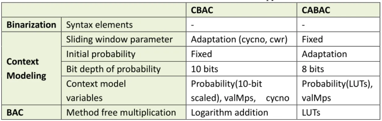
Table 3- 1 The differences between two entropy coders ... 36

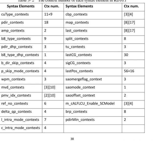
Table 3- 2 The context number of each syntax element in RD10.1 ... 38

Table 3- 3 the performance comparison result of CABAC with CBAC ... 42

Table 4- 1 The approximation error compensation table ... 46

Table 4- 2 The coding efficiency using approximation error correction tables ... 48

Table 4- 3 The model variables for the probability estimation ... 51

Table 4- 4 The BD-rate of proposed probability estimation with RDOQ-off ... 57

Table 4- 5 The BD-rate of proposed probability estimation with RDOQ on. ... 57

Table 4- 6 The BD-rate of using rate estimation (2-bit and 8-bit fraction part).... 62

Table 4- 7 The time saving when the rate estimation table is used in AVS2.0 ... 62

Table 5- 1 Summary of the implementation result ... 77

(13)

List of Figures

Figure 1- 1 The typical video codec block diagram ... 1

Figure 1- 2 The development of video codec standard ... 3

Figure 1- 3 The coding block diagram of AVS2.0 ... 3

Figure 1- 4 The quad-tree partition structure in AVS2.0 ... 5

Figure 1- 5 The prediction unit structure in AVS2.0 ... 6

Figure 1- 6 Intra prediction direction in AVS2.0 ... 6

Figure 1- 7 scheme for comparison between two entropy coders. ... 10

Figure 2- 1 The general block diagram of CBAC in AVS2.0 ... 17

Figure 2- 3 Subdivision and decision procedure of BAC ... 22

Figure 2- 4 One binary arithmetic coder cycle ... 24

Figure 2- 5 The slice coding structure for the CBAC ... 28

Figure 2- 6 Sub-block scan: each sub-block is a Coding Group (CG) ... 29

Figure 2- 7 4*4 Coefficients scan within a CG ... 29

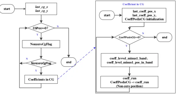
Figure 2- 8 Coding flow for the transform coefficients ... 31

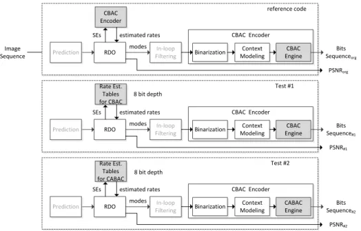
Figure 3- 1 The Block Diagram for Evaluating CBAC and CABAC Engines ... 37

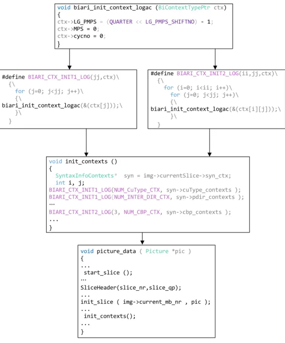
Figure 3- 2 the context initialization procedure in RD10.1 ... 39

Figure 4- 1 The flowchart of CBAC encoder ... 54

Figure 4- 2 The proposed probability estimation scheme for each context model.56 Figure 4- 3 The block diagram of proposed rate estimation ... 58

(14)

Figure 4- 4 Probability distribution of the CABAC range ... 59

Figure 4- 5 The BD-rate changes with different fraction part lengths ... 63

Figure 5- 1 the General BAD Structure in AVS2.0 ... 65

Figure 5- 2 The overall structure for the BAD with one-bin scheme ... 66

Figure 5- 3 Flow chart of rangeI update ... 67

Figure 5- 4 Flow chart of rangeF update ... 68

Figure 5- 5 Detailed Structure of Module for Range Update ... 69

Figure 5- 6 offsetI update block diagram ... 70

Figure 5- 7 flow chart of updating offsetF ... 71

Figure 5- 8 Offset Update logic diagram block ... 72

Figure 5- 9 Bits Read Logic Block Diagram ... 73

Figure 5- 10 The process of Context Updating in the CBAC decoder in AVS2.0 .. 75

Figure 5- 11 Detailed Structure of Module for Context Update ... 76

(15)

Chapter 1 Introduction

1.1 Research Background

Recent years, with the rapid development of the information technology, the demand for the multi-media, such as video media, is getting greater and greater.

Mass data offered by the video carrier make the information storage and transmission more difficult to handle and it is necessary to explore the effective and efficient video compression technique, especially in the vast images data and real- time transmission with high definition requirement. The video compression and coding technique has been significantly enhanced since it merged in 1980s. The main procedure of video codec includes prediction for video images to obtain the residual data, transform and quantization for the residual data, entropy coding for the data after quantization, as well as the bit-stream collection finally. However, a reverse procedure is performed for the decoder part, and the reconstruction video sequence is achieved through bit-stream as input. The typical video codec structure can be described as Fig.1-1.

Image

Segmentation Prediction Transform Quantization Entropy Coding Video

image

bit-stream

Entropy Coding Quantization

Transform Prediction

Image Segmentation Recon.

image

Encoder

Decoder

Figure 1- 1 The typical video codec block diagram

(16)

Many efforts have been made by the video expects from the International Telecom Union (ITU) , Video Coding Expert Group (VCEG), International Standard Organization (ISO) and Moving Picture Expert Group (MPEG) in the past several decades and consequently there are considerable development in the video compression standards. H.261 is the first generation motion image compression standard developed by the ITU^[1] followed by the H.263 standard proposal[2] which was developed for the low bit rate video coding at the Nov. 1995. H.263 was aimed to the low bit rate compression for the high quality motion image and used to support the application with bit rate less than 64kbits/s. In the following several years, ITU proposed couple improved vision based on H.263. IMEG family [3]

including MPEG-1, MPEG-2, MPEG-4, MPEG-7, and MPEG-21 have been developed by the ISO. Until at the beginning of the 21-st century, H.264/AVC [4]

introduced by the ITU and ISO brought about 50% performance improvement compared with MPEG-2 and has been popular in the industrial application. At the same time, another video standard, named AVS[5] developed by the Audio Video coding Standard (AVS) Workgroup in China. The coding complexity was deduced compared with the H.264/AVC with a comparable coding efficiency. Along with the new high definition and ultra-high definition video requirements, High Efficiency Video Coding (HEVC) [6] were proposed and finished the final draft in 2013 by the Joint Collaborative Team on Video Coding (JCT-VC) which is the cooperative team including ITU VCEG and ISO MPEG. This standard has been designed aim to save over 50% [7] bit rate to get the comparable quality, albeit at

(17)

higher computational costs. Correspondingly, AVS workgroup has spared more efforts to make second generation video codec orientated to higher coding efficiency referred as AVS2.0 [8]. Specifically, the video technique can be represented as the Fig.1-2 according to the development in the past 30 years.

1990 2000 2010

Technology background

MPEG1

H.261 H.263

MPEG 2 HEVC

AVS2

H.264/AVC, AVS VP9

Figure 1- 2 The development of video codec standard

1.2 Key Techniques in AVS2.0

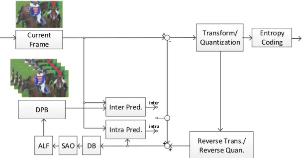
Similar with other mainstream video coding standard, the overall coding framework of AVS2.0 can be shown in Fig.1-3.

Current Frame

DPB

Transform/

Quantization

Entropy Coding

Reverse Trans./

Reverse Quan.

+ -

Inter Pred.

Intra Pred.

inter

intra

DB SAO

ALF ⁺ ₊

Figure 1- 3 The coding block diagram of AVS2.0

(18)

However, the specific techniques introduced into AVS2.0 standard includes Intra prediction, Inter prediction, Transform & Quantization, Entropy coder, Sample adaptive offset, and Adaptive loop filter [9]. With the similar algorithm structure of HEVC, AVS2.0 has the competitive coding efficiency but more simplified algorithms for each mode to deal with video image. Although the coding procedure of AVS2.0 shares the similar structure of HEVC, AVS2.0 pays more attention on some special application scene, such as surveillance video, real-time video meeting, etc. Specifically, for each part, including Intra prediction, Inter prediction, Transform/Quantization, Entropy coding and Loop filter, technique baseline and performance improvement in BD-rate saving (%) in AVS2.0 are presented in Table 1-1.

Table 1- 1 Key techniques used in AVS2.0

Type Technique baseline Coding

gain Image

structure

Hierarchical reference frame

B picture used as reference

Forward multiple hypothesis

prediction picture

8% ~ 13%

Block structure

Quad-tree based coding unit partitions

Non-square intra prediction

Non-square inter prediction

Non square

transform

15% ~ 20%

Intra prediction

33 directional prediction modes

1/32 sub pixel prediction

5% ~ 10%

Inter prediction

Forward multiple hypothesis prediction, special prediction mode and motion vector prediction

Progressive motion vector coding

DCT like

interpolation filter

7% ~ 12%

Transform

Multiple size and highly normalized integer transform

Secondary transform 3%

Entropy

coding Two level scan coding 5%

Loop filter Deblock filter Sample adaptive offset Adaptive loop filter 8%

(19)

Then we will briefly introduce the key feature of each technique adopted in AVS2.0.

A. Block Structure

The block partition is more adaptive compared with AVS1.0 by using quad-tree structure. The 64*64 is the largest coding unit (LCU) and then it is partitioned into smaller coding unit (CU) until reaching the minimum coding unit limitation size 8*8. Through this partition mode, then coding tree (CTU) structure is obtained.

Fig.1-4 gives the quad-tree partition structure.

Figure 1- 4 The quad-tree partition structure in AVS2.0

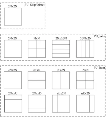
Each CU then can be divided into some prediction unit (PU), PU is the basic unit for intra and inter-picture prediction. For intra prediction, there are four type PUs among which N*N PU is used for 8*8 CU only and 2N*0.5N/0.5N*2N are introduced in CU size 32*32 and 16*16. Eight types PU are used in inter prediction, including 2N*2N、N*N、N*2N、2N*N、2N*nU、2N*nD、nL*2N、nR*2N. The maximum PU size is decided by the current CU and minimum PU is 4*4. The transform unit (TU) is another coding block which is used for the transform and quantization operations. TU is also decided by the current CU size without consideration the PU size anyway, 64*64 and 4*4 are the maximum and minimum TU size, respectively. Fig.1-5 is the prediction coding unit partition structure.

(20)

2Nx2N PU_Skip/Direct

2Nx2N PU_Intra

NxN 2Nx0.5N 0.5Nx2N

2Nx2N PU_Inter

2NxN Nx2N NxN

2NxnU 2NxnD nLx2N nRx2N

Figure 1- 5 The prediction unit structure in AVS2.0 B. Intra Prediction

Intra prediction is employed to remove the spatial redundancy within picture. Multi- direction intra-picture prediction is used in AVS2.0 and as described in A section, except for four partitions, the Short Distance Intra Prediction (SDIP) [10] is used for intra prediction on 32*32 and 16*16 CU. Fig.1-6 shows 33 modes including DC, Plane, Bilinear and 30 Angle modes for luma component.

Figure 1- 6 Intra prediction direction in AVS2.0

18 6

30

22 20

16 14 10 8 4

26 28 32

23

21

15 19 17

11 13

9 7 5 3

25 27 29 31

12

24

DC: 0 Plane: 1 Bilinear:2 zone1

zone2 zone3

(21)

C. Inter Prediction

Inter prediction is employed to remove the spatial redundancy between picture.

AVS2.0 uses 8 inter prediction modes as described in A section, and 3 frame types:

P frame, B frame, and F frame. F frame is developed based on the P frame with bi- forward inter prediction. In inter prediction, there are specific techniques patented by AVS2.0 developer group, including Dual Hypothesis Prediction (DHP) [11], Directional Multi-Hypothesis Prediction (DMH) [12], Progressive Motion Vector Resolution (PMVR) [13], etc.

D. Transform & Quantization

In AVS2.0, the two-level transform coding to deal with residual data. Firstly, using Wavelet Transform and then DCT transform as the TU size is divided into 32*32.

In DCT transform, 4*4 ~ 32*32 TU size are supported and Non-Square Quad-tree Transform (NSQT) is used to handle non-square TU. In order to reduce the information redundancy, the residual data will be performed a second DCT transform [14].

In addition, Rate Distortion Optimization Quantization (RDOQ) is another technique adopted by the AVS2.0 in the rate distortion optimization process. RDOQ makes the compromise between the computation complexity and the coding efficiency. To reduce the complexity to decide mode, only is the mode within the one coding unit decided, the RDOQ is used for the coefficients quantization in the best mode in AVS2.0.

(22)

E. Entropy Coding

The entropy coding in AVS2.0 is only context-based binary arithmetic coding (CBAC), which is different from AVS1.0 where CBAC and variable length coding technique are performed as entropy coders. In CBAC, two-level transform coefficient coding scheme acts as the well-designed entropy coding strategy. The two-level scheme [15] employs the similar concept of sub-block based partition as in HEVC and applies this scheme to the (Level, Run) coefficients pair of large blocks. In this scheme, the sub-block size is set to a fixed value with 4×4 and named as one coefficient group (CG) in the following text.

Entropy coding plays a vital role in the entire coding structure as the Fig.3 illustrates.

It locates in the last step of the encoder and the first step of decoder which determines the bin-to-bit compression ratio which is relative the coding performance. Entropy coding, especially CBAC is the study center in this research topic, and more detail will be shown in the following several chapters.

F. Loop Filter

To reduce the visual flaw caused by the video coding algorithm, there are three methods used in AVS2.0 including Deblocking Filter (DF), Sample Adaptive Offset (SAO) [16], and Adaptive Loop Filter (ALF) [17] to address the visual problem for the reconstructive picture.

Even through a significant compression efficiency has been achieved by AVS2.0 based on the above techniques compared with AVS1.0, the improvement in each

(23)

technique perspective can be explored to make it better enough to comparable with other popular video coding standard, such H.264/AVC, HEVC etc. However, in order to escape the copyright and patents own by other standards, the techniques employed in AVS tend to be more complexity and simpler in the algorithm implementation. Thus, the study on the AVS2.0 is full of challenge in the algorithm design and schedule implementation practically.

1.3 Research Contents

In AVS2.0, context-based binary arithmetic coding (CBAC) [18] is the only entropy coding method introduced into current standard. In this thesis, there are three topics we focus on the entropy coder CBAC in AVS2.0. Firstly, we compare performance between two entropy coder with different algorithm, which are CBAC and context- based adaptive binary arithmetic coding (CABAC) that is used in H.264/AVC and HEVC. Secondly, we propose some ideas about the CBAC performance enhancement and then introduce the fast rate estimation model for the AVS2.0 in the rate distortion optimization (RDO) mode decision process. Lastly, we implemented Binary Arithmetic Decoder with throughput of one-bin per cycle, which is main bottle-neck of implementation of CBAC Decoder with high throughput. More detail will be shown in the following several subclasses.

1.3.1 Performance Comparison of CBAC

We propose a fair scheme to compare the CBAC with Context-based Adaptive Binary Arithmetic Coding (CABAC) [19] in HEVC, as Fig.1-7 shows, we implant

(24)

CABAC logic that is designed for HEVC into RD10.1, which is one of latest versions of reference software of AVS2.0. The coding efficiency of AVS2.0 using two entropy coders can be evaluated by bitstream 0 and bitstream1, which are from the result of encoding the given video sequence.

Intra/Inter prediction

Transform/

Quantization

CBAC

CABAC RD10.1

bitstream0

bitstream1 Image Seq.

Figure 1- 7 scheme for comparison between two entropy coders.

Through comparison of these two entropy coders, we can obtain the knowledge about entropy coding compression performance. Our evaluation experiments show that CBAC algorithm tend to be more efficient than CABAC with about 0.4% BD- rate saving when we use the CABAC algorithm of HEVC directly to encode the same video sequences.

1.3.2 CBAC Performance Improvement

With understand of the reason of coding efficiency improvement, we explore more in CBAC algorithm in AVS2.0. Most of algorithms in Codec are usually used to implement without using multiplier operation to reduce Complexity of Computation.

In the process of updating variables, which is used for Arithmetic Coding such as range and context probability, multiplier operations are replaced with other operations similarly. Look-up table is used in CABAC in HEVC for the purpose of

(25)

this. While the logarithm addition and shift operations is used in CBAC. But, introduction of operation of logarithm domain necessarily accompany the process to convert data between real domain and logarithmic domain, which requires additional computational complexity. So CBAC uses two approximation equations to minimize overhead by domain conversion. For that reason, it is likely to increase coding performance if we can reduce approximation error at the sake of minimal increase of computational complexity.

Therefore, we present compensation tables to minimize the error by approximation equations within the CBAC engine by introducing adjusted factors when the approximation equations are used in domain conversion.

Adaptive probability estimation [20] [21] is another topic in CBAC which is a powerful optimization to indict how to map the symbol statistical behavior. Based on the fact that probability estimation in CBAC is also performed in the logarithm domain with probability in certain bits resolution, we explore the probability estimation scheme with the perfect bit resolution and well-designed update process.

In addition, rate estimation is introduced into AVS2.0 in order to save the overall encoding time. Different from AVS2.0 software reference, we use the proposed rate estimation table to support the rate distortion cost in the Rate-Distortion Optimization (RDO). Though the proposed rate estimation model, the encoding time can be reduced about 1% without considerable performance degradation.

(26)

1.3.3 Implementation of Binary Arithmetic Decoder in CBAC

Through the above two chapters in the algorithm study, we understand the software implementation detail better. Based on this understand, the hardware-oriented architecture for binary arithmetic decoder is described in this chapter. Considering the total CBAC decoder will cost more time to arrange reasonable context models, only Binary Arithmetic Decoder (BAD) with one bin scheme is designed in this chapter, but we give the proposed context update module architecture. For the BAD, there are three important loops needed to update after one bin is decoded, which includes range update loop, offset update loop and bits read. Correspondingly, we design three modules to realize the update: range update module, offset update module, bits read module. Since few previous work is focus on the CBAC decoder in AVS2.0, we compare our work with the available CBAC decoder design in AVS1, and the competitive result can be achieved based on our BAD architecture.

1.4 Organization

Chapter 2 describes the entropy coding CBAC in AVS2.0 and how it works the arithmetic engine. Also, the two-level transform coefficients coding is given in detail. In Chapter 3, the coding efficiency of CBAC and CABAC of HEVC are compared based on the software platform of AVS2.0 RD10.1. We proposed a quite fair comparison scheme with consideration of initial context variables, binarization, adaptive probability estimation model, etc. In Chapter 4, we propose some idea to improve coding efficiency in CBAC such as error compensation, new probability

(27)

to implement binary arithmetic decoder in CBAC in Chapter 5. In the last Chapter, the research conclusion about this thesis and further research orientation are posted.

(28)

Chapter 2 Entropy Coder CBAC in AVS2.0

2.1 Introduction of Entropy Coding

Context-based Adaptive Binary Arithmetic Coding (CABAC) is a method of entropy coding first introduced in H.264/AVC, and it is also adopted in the newest standard - High Efficiency Video Coding (HEVC). Similar with the method used in above standards, another kind of entropy coding approach – Context-based Binary Arithmetic Coding (CBAC) is introduced in a Chinese video standard – Audio and Video coding standard (simplified as AVS) by the Audio Video coding standard of Workgroup of China. However, the strong data dependence and serious operations in nature make entropy coding more complicate to parallelize and improve the throughput. Thus in the design of standard of entropy coding for H.264/AVC, HEVC, and AVS, the balance of coding efficiency and throughput should be considered.

Specifically, all the current entropy coding engines are based on the arithmetic coding [22] [23]. Arithmetic coding is different from other coding methods because we know the exact relationship between the coded symbols and the actual bits that are written to a file. It codes one symbol once, and a real-valued number of bits is assigned to each symbol. The code value v of a compressed data sequence is the real number with fractional digits that equals to the sequence’s symbol. We can convert sequence. This construction create a convenient mapping between infinite sequences of symbols from a D-symbol alphabet and real numbers in the interval [0, 1), where any data sequence can be represented by a real number, and vice-versa. This kind of code value

(29)

presentation can be used in any coding system, and it makes a universal method to represent large amounts of information of a set of symbols used for coding, such as binary, decimal, etc. By analyzing the distribution of the code value it produced, we can evaluate the efficiency of any compression method. According to Shannon’s information theory, we can know that, if a coding method is optimal, then the code values cumulative distribution has to be a straight line from point (0, 0) to the point (1,1). When it is applied into video coding, it is attached with context information of each symbol. Therefore, entropy coding is the kind of lossless compression approach which can use the statistical probabilities of source information, e.g. video or image carriers, so that a string of bits can be used to represent the symbols is logarithmically proportional to the corresponding probability of each symbol. When compressing a string of symbols, the symbol which occurs in a large frequency can be represented by few bits, while the other symbols with less frequent emergence, represented with a longer bit string. According to the Shannon’s information theory, the probability of a symbol represented in bit 0 or 1 is p, the optimal average code length for one symbol is –log₂ p.

In the general videoing coding standard, the classical codec framework is represented as Fig.1. And the entropy coding is performed in the last step of the overall video coding after the video signal has been parsed to series of syntax elements. Correspondingly, it is in the first stage of the video decoding procedure in each standard.

(30)

2.2 CBAC Overview

The CABAC algorithm is firstly introduced within the joint H.264/AVC standard of ITU-T Video Coding Experts Group (VCEG) and ISO/IEC Moving Picture Experts Group (MPEG). CABAC was used as one of two alternative methods of entropy coding in H.264/AVC, and introduced as the only method in HEVC.

Similarly, the entropy coding in AVS 1.0 jizhun file includes two schemes, C2DLVC and CBAC, which not only adopted 2-dimension (run, level) coding scheme used in MPEG-2, but also absorbed the context-based adaptive binary arithmetic coding strategy used in H.264/AVC. In C2DVLC, the VLC multiple tables achieved by training in off-line. It is not able to capture the local statistical distributions in nature and a symbol with a probability which is greater than 0.5 cannot be coded efficiently considering the nature limit to 1 bit/symbol in VLC codes. However, the arithmetic coding can challenge this restriction with a higher coding efficiency.

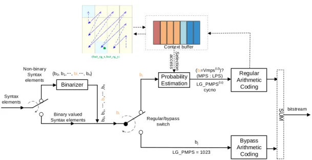
Therefore, in this section, the CBAC algorithms and separated key technique are represented systemically from the AVS1.0 to AVS2.0. The general procedure for the CBAC includes binarization, context derivation and selection, and arithmetic coding engine. And these compounds illustrated in Fig.2-1. The binarization process is aimed to translate the values of the non-binary syntax elements into binary and it is defined as the bin string generation process. The context derivation and selection process is related to the probability modeling process, in which the each bin can be mapped into a specific context to estimate the probability of each regular bin. Finally, the binary arithmetic

(31)

information and probability distribution. There are two kinds of the arithmetic coding paths according to the probability value for each bin, including the regular path and bypass path.

Binarizer

Probability Estimation Context buffer

Regular Arithmetic

Coding LG_PMPS^(I,t)

cycno Non-binary

Syntax elements

Bypass Arithmetic

Coding {b0, b1,…, bi,…, bn}

bi b0, b1, …, bi,… ,bn Syntax

elements

Binary valued Syntax elements

bi

Regular/bypass switch

(bi=Vmps^(i,t))?

(MPS : LPS)

b_j LG_PMPS = 1023

SUM

bitstream

Selection access

Figure 2- 1 The general block diagram of CBAC in AVS2.0

2.2.1 Binarization and Generation of Bin String

Binarization process is aimed to uniquely map process of all possible values of a syntax element onto a set of bin string. For the non-binary valued symbols, e.g. Level and Run, they should be performed the binarization process as the values of this kind of syntax elements tend to be typically in a large range in a DCT block. When this value is coded directly by the m-ary (m>2) arithmetic code, it will have a high computation complexity.

Moreover, the source with typically large alphabet size often suffers from “context dilution” effect when the high-order conditional probabilities have to be estimated on a relatively small set of coding samples. In addition, the context modeling for the sub syntax element level provides more accurate probability estimation than that in the

(32)

syntax elements level, and the alphabet of the encoder is decreased.

There are several methods of binarization adopted in video coding standard. All of these methods, including Unary, Truncated Unary, k-th order Exp-Golomb (EGk), and Fixed length are introduced to reduce the alphabet size of syntax elements to encode.The binarization methods for syntax elements which are applied into the CBAC of AVS2.0 represented as the following [24]:

(1) Unary coding is used to binarize the symbol into a bin string with length N+1, including the first N bins with value 1 and the last bin is 0.

(2) Truncated Unary scheme is defined based on the largest possible value maxVal of the syntax element. Before maxVal, the binarization value is the same as the Unary, and when the value is equal to maxVal, all the bins in the bin string are set to 0 and the total bins are the same as that of the maxVal -1.

(3) Marking bit is defined as the bin value is the same as the value of the syntax element.

(4) The k-th order Exp-Golomb coding with k ranged from 0, 1, 2, 3, has a general construction, which consists of a prefix and suffix. For the given codeNum N and the specific order k, the code word consists of l zeros followed by one 1 and suffix of N-2^k(2^l-1), and the l is defined as following:

However, except for the above several schemes, for most syntax elements in CBAC, the binarization process is defined based on the type of the syntax element.

(33)

2.2.2 Context Modeling and Probability Estimation

Context Modeling Process, shown in Fig.2-1, consists of three sub steps: context model derivation, context model selection andcontext model access. The context modeling process is referred as the probability selection process. In the regular binary arithmetic coding process, where the probability model is decided by the fixed modelbased on the type of the syntax elements and the bin position or the bin index in the binarized representation of the syntax elements. Another kind of context (probability model) is adaptively chosen from the two or more than two probability models according to the side information, such as the special neighbors(Left, Above block), components (Luma, Chroma), depth and size of the CTU, PU, TU as well as the position of within one TU.

The adaptive case is generally adopted into the observed bins with high frequency while the fixed model is usually applied for the less frequently occurred bins. Thus the modeling process can be benefited from the balance of the choice cost and context learning complexity with the estimated accuracy.

Similar with probability models in CABAC adopted in H.264/AVC and HEVC, the CBAC probability updating model is based on the adaptive probability model as well, in which the parameters of the probability model make a promising contribution to the map the statistical variations of the source bins which is performed bin-by-bin basis as the sub symbol. This is the probability estimation process. The derivation of the CBAC probability updating process is applied for the infinitely independent identical distribution (IID) [25] of the binary source. If the probability of the symbol “1” is p, and the probability of the symbol “0” is q. And the adjusting parameter N is defined to

(34)

adjust the updating speed. Then

p

_kand

q

_kare defined as the estimated probability of the symbol “1” and “0” after the k-th iteration. And then we can achieve the probability after (k+1)-th iteration as the following equation 2-1:

1

( "0" ) 1

( "1" ) 1

k k

p N p if occurs

N

q N q if occurs

N



  

 

 

 

 



(2-2)

According to the relationship between p and q, i.e.

p

_k

  1 q

_k, the equation (2-2) can be changed as the following equation (2-3):

¹

1

( "0" ) 1

1 ( "1" )

1 1

k k

p N p if occurs

N

p N p if occurs

N N



  

 

 

  

  



(2-3)

According to the above equations, the expectation and variance of the

p

_k_₁are proved to converge to a constant value which is dependent on N. Therefore, if we use the

p

_MPS

and

p

_LPS as the probabilities of the MPS and LPS symbol, thus the probability change can be obtained based on the equation (2-2), as the following equation (2-4):

( )

MPSnew MPSold

LPSnew LPSold

LPS MPS

p p if occurs

  

  





 (2-4)

Here 1

N

 N

  . That is to say, the larger the N is, the α is smaller, the slower the estimation converges, the variance is smaller, thus the probability estimation is more accurate.

However, in H.264/AVC and HEVC, the probability estimation model is based on the assumption that the estimated probabilities of each context model can be represented by a sufficiently limited numbers of representative values. For the CABAC engine,

(35)

there are 64 limited representative probability values p, which is ranged from 0.01875 to 0.5, including. The estimation model can be derived from the recursive equation of the LPS symbol as the following (2-5):

p

_δ

  α p

_{δ 1}_

( δ 1, 2 , 3 , . . . , 6 3 ) 

(2-5) With α (^0.01875)^1/63 ₀ 0.5

0.5 and p

 

The scaling factor α ≈ 0.95 and the probability state is set as 64, in which the compromise of the speed and estimation accuracy. Each probability

p

_δ is addressed according to the probability state.

As to the practical implementation procedure, In CABAC of H.264/AVC and HEVC, the probability state updating process is based on the 64-state Finite State Machine (FSM). In this process, the state transfer process is performed to index a pre-defined state table, where the state is the index, and state is also the key variable for each context.

Similarly, In AVS1 and AVS2.0, the context modeling adopts the same probability estimation model to model the information source and performing probability updating process for each context. However, since CBAC and CABAC apply different schemes to perform the entropy coding, the probability modeling process is experienced various procedure, especially in the term of practical implementation. In AVS, the state of probability estimation model is based on the logarithm value of probability, which is scaled into 10-bit resolution domain (0 ~ 1024) in theory. Therefore, the probability model is based on the probability and logarithm value of the probability of MPS symbol.

The scaled probability LgPmps can be described as equation (2-6):

(36)

Here, pmps is the MPS probability. Thus for each probability including MPS and LPS are indicted in the scaled probability LgPmps when it implemented in CBAC. The statistics of the coded syntax elements are utilized to update the probability models, which is related to context models of regular bins. Therefore, more specific explanation of the transition rules for updating the state indices will be shown in binary arithmetic coding, and contexts design derivation sections.

2.2.3 Binary Arithmetic Coding Engine

The basic principle of arithmetic coding is introduced in [22], which is based on the recursive interval subdivision of the interval width R. Each binary symbol of the information source which is represented by a bin string, associated with a specific context model, which keeps update during the coding process in order to adaptively estimate the probability. Therefore, the variables for BAC is bin value, slice type, and the context model for each bin. And BAC is a recursive process of the coding interval (range, offset, low) subdivision, updating, and renormalization operations as Fig. 2-2.

Figure 2- 2 Subdivision and decision procedure of BAC

A given interval initially which can be represented as the lower bound L and range R is C

(37)

subdivided into two sub-ranges according to an relative estimation of the probability plpsvalued from 0 to 0.5, not including, of the Least Probability Symbol (LPS).Thus another part can be described as p_mpsand subrange R_mpsof Most Probability Symbol (MPS). One of the sub-range can be denoted as the following equation:

Which is associated with the MPS symbol and corresponding interval of the range LPS

lps mps

R  R R , which is related to the MPS with a probabilityp_mps  1 p_lps. According to the binary value to be encoded, the relative LPS or MPS range will be chosen as the new interval for the next iteration.

Based on the above description, the subdivision is performed via the multiplication, but multiplication operation is proven with high computation complexity and calculation cost both in software and hardware. The practical implementation method has been focus on the multiplication-free operations, such as the look-up table approach which is used in H.264/AVC and HEVC, where a well-developed table is pre-designed, the sun-range can be obtained from the look-up table operation. Thus the multiplication operation is eliminated. However, the CBAC in AVS2.0 is based on a novel algorithm which is based on the domain conversion between logarithm and original domain. By this method, the multiplication operation can be substituted by the logarithm adder operation in logarithm domain. More detail about the two methods to reduce the multiplication complexity will be represented in the following sections.

In CABAC, the BAC is performed on the look-up table to realize the range subdivision

(38)

and applies for the FSM to deal with the state transition for the context and probability updating. However, the procedure in CBAC in AVS2.0 experience a various scheme.

The process is an iterative one which consists of consecutive MPS symbols and one LPS symbol. 9-bit precision for range is kept during whole coding process. In the binary arithmetic coder of CBAC, we substitute the multiplication in (2-7) with addition by using logarithm domain instead of original domain. When a MPS happens, the renewal of range is given as

where Lgx indicates the logarithm value of variable x and LgR_mps is the new range after encoding one MPS. For the case of encountering one LPS, we denote the two MPS range before and after encoding the LPS as R1 and R2 as shown in Fig. 2-3. Then, the range after the whole coding cycle in original domain should be

R_lps  R₁ R₂ (2-9)

range

R1

R2

LPS

MPS MPS

MPS

low_new

low

Figure 2- 3 One binary arithmetic coder cycle

And the new lower bound of current range equals to the addition of low and R2. Since

(39)

R1 and R2 are both calculated on the logarithm domain, we have to get the value of R1

and R2 from

LgR

₁ and

LgR

₂, and then

and

Here,

s s

₁ ₂ are the integer, and t t₁ ₂ are the fraction part, which range from [0, 1). Δ1

and Δ2 are the approximation error adjust factor. From (2-10), (2-11), we can get the following, ignoring the approximation error Δ1 and Δ2:

R_{l p s}2^^s¹t₃ (2-12) and

² ¹

2 1

1 2

3

1 2

( )

( 1)

f s s

t t i

t t t i



 

 

    (2-13)

After the new value of R_lps is obtained, the renewed lower bound is updated. Then the renormalization process is carried out to guarantee that the most significant bit of the updated range value is always ‘1’. Until now, one coding cycle is finished. After one bin is encoded by arithmetic coder, the estimated probability of the chosen context should also be updated. In order to prepare the relative parameters for the next iteration, the range in original domain should be exchanged into logarithm domain. Considering a fact that the approximation will stand when the variable x ranged into a small interval (0, 1) as following:

ln(1x)x (0 x 1) (2-14)

(40)

The integer part of the logarithm-based updated range R_lpss1 is 0, and the fraction part

t

₃ can be simplified with the above equation. Thus the R_lps in logarithm domain can be obtained and the range preparation for the next cycle is finished.

Actually, in CBAC, the probability of each context model is set to be 0.5 for both MPS and LPS at the start of coding initially. With the coding of some bins, the adaptive probability estimation of MPS on logarithm domain is performed. Based on the context modeling section described in section 2.2.2, the practical probability estimation is fulfilled using only additions/subtractions and shifts as in the following formulas:

⁽ ⁾

( ) ( )

LgPmps LgPmps Lgf if lps

LgPmps LgPmps LgPmps cw if mps

 

   

 (2-15)

Where f is equal to (1-2^-cw). Here, cw is the size of sliding widow to control the speed of probability adaptation. The smaller cw is, the faster the probability adaptation will be. In the practical implementation process, the cw is adaptive according the cycno parameter, which is adopted to record the iteration of calling the CBAC engine.

2.3 Two-level Scan Coding CBAC in AVS2.0

Different from AVS1, AVS2.0 supports larger transform blocks (e.g., 16×16 and 32×32).

In the early stage of AVS2.0 standardization process, the CBAC design for AVS2.0 is inherited from that in AVS1 by a straightforward extension. However, CBAC was primarily designed for 8×8 transform blocks while the non-zero coefficients may be sparser in larger transform blocks. Therefore, to further improve the coding efficiency

(41)

and throughput issue in hardware implementation, AVS2.0 CBAC employs a two-level coefficient coding scheme [15].

Generally, the iteration of CBAC in AVS is slice, which means that all the binary arithmetic coding engine relative parameters will be initialized after finishing one slice.

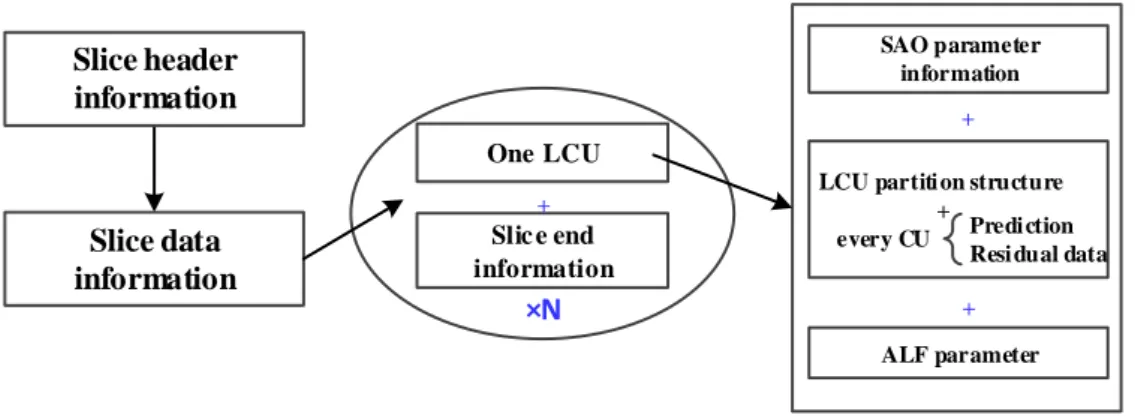
Only the syntax elements which are belong to the slice segment data, will be processed by the CBAC encoded. The coding structure in the slice illustrated as Fig.2-4, including slice header information, slice data information, the coding procedure in one LCU, and the slice end information. The syntax elements that are coded with CBAC in AVS2.0 include three categories: (1) context-based syntax elements, (2) bypass mode-based syntax elements, (3) stuffing bit-based syntax elements. For AVS, these context-based syntax elements describe the properties of the coding tree unit (CTU/LCU), coding unit (CU), prediction unit (PU), and transform unit (TU). For the CTU level, the related syntax elements are used to represent the block partition information of the CTU, the type including edge and band, and offsets for the sample adaptive offset (SAO), and adaptive loop filtering in loop filtering in CTU. For a CU, the syntax elements are related to describe whether the CU is intra prediction mode, or inter prediction mode, the PU type definition of B and F frame. For a PU, it includes the syntax elements which describe the intra prediction mode, and the motion data. For the TU level, the coding tree pattern, and residual data including transform coefficient, level and run information.

(42)

×N Slice header

information

Slice data information

One LCU

Slic e end information

LCU partiti on structure +

every CU SAO parameter

information

+

Predi ction Resi dual data

ALF parameter +

Figure 2- 4 The slice coding structure for the CBAC

However, entropy coding in AVS, which is the similar with CABAC in H.264/AVC and HEVC, provides a high coding efficiency, while its strong data dependence caused by the serious operations in its procedure put a big challenge on the throughput improvement. The throughput of CBAC is determined by the binary symbol that it can be performed per second. Moreover, the significant contribution is made by the syntax elements of transform coefficient data, which includes the residual of the prediction error.

The two-level scheme employs the similar concept of sub-block based partition as in HEVC [26] and applies it to the (Level, Run) coding to address the spatiality of large blocks. In this scheme, the sub-block size is set to a fixed value, i.e., 4×4. Such a sub- block is named one coefficient group (CG) in the following text. The CG level coding is firstly invoked, followed by the (Level, Run) coding within one CG which is similar to CBAC in AVS1.

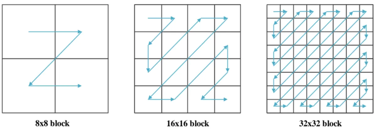
2.3.1 Scan order

In CBAC for AVS2.0, the coefficient coding for a transform block (TB) is decoupled

(43)

into two levels, i.e., CG level coding and coefficient level coding. In both levels, the coding follows the reverse zig-zag scan order. Fig. 2-5 shows the zig-zag scan pattern in a TB with a different size, which is split into sub-blocks and the scan order of CGs is indicated by lines while the scan order within one CG is indicated as the line shows in Fig.2-6. The CG-based coding methods have two main advantages:

 Allowing for modular processing, that is, for harmonized sub-block based processing across all block sizes.

 With much lower implementation complexity compared to that of a scan for the entire TB, both in software implementations and hardware.

8x8 block 16x16 block 32x32 block

Figure 2- 5 Sub-block scan: each sub-block is a Coding Group (CG)

16x16 block 16 coefficients in a CG

Figure 2- 6 4*4 Coefficients scan within a CG

(44)

2.3.2 First level coding

For the current coding block which is divided into multiple CGs as Fig.2-5 shows. The first level coding is performed among these CGs. At inter CG level, the position of the last CG is signaled, where the last CG is the CG that contains the last non-zero coefficient in the transform block in the scan order. Different ways are used to signal the position of the last CG which is dependent on the TB sizes. For an 8×8 block, a syntax element LastCGPos is coded, which is the scan position of the last CG. For larger TBs, such as 16×16 and 32×32 TBs, one flag LastCG0flag is firstly coded first to indicate whether the last CG is at position (0, 0). In the case that lastCG0flag is equal to one, two more syntax elements LastCGX and LastCGY are coded to signal the(x, y) coordinates of the last CG position. Note that, (LastCGY- 1) is coded instead of LastCGY when LastCGX is zero since lastCG0flag is equal to one.

The first level coding is performed by several syntax elements which indicate the information about the current CG in the entire TB. Thus the syntax elements for this level are explained by the last_cg_pos, last_cg0_flag, last_cg_x, last_cg_y, last_cg_y_minus1 and nonzero_cg_flag and each description is presented in Table 2-1.