저작자표시-비영리-변경금지 2.0 대한민국 이용자는 ... - S-Space

저작자표시-비영리-변경금지 2.0 대한민국 이용자는 아래의 조건을 따르는 경우에 한하여 자유롭게

l 이 저작물을 복제, 배포, 전송, 전시, 공연 및 방송할 수 있습니다. 다음과 같은 조건을 따라야 합니다:

l 귀하는, 이 저작물의 재이용이나 배포의 경우, 이 저작물에 적용된 이용허락조건 을 명확하게 나타내어야 합니다.

l 저작권자로부터 별도의 허가를 받으면 이러한 조건들은 적용되지 않습니다.

저작권법에 따른 이용자의 권리는 위의 내용에 의하여 영향을 받지 않습니다. 이것은 이용허락규약(Legal Code)을 이해하기 쉽게 요약한 것입니다.

Disclaimer

저작자표시. 귀하는 원저작자를 표시하여야 합니다.

비영리. 귀하는 이 저작물을 영리 목적으로 이용할 수 없습니다.

변경금지. 귀하는 이 저작물을 개작, 변형 또는 가공할 수 없습니다.

공학박사 학위논문

Generation Mechanism and

Machine-Learning Forecasting Model of Sudden High Waves in the East Sea

동해 돌연고파의 발생 메커니즘과 기계학습 예측모델

2017년 08월

서울대학교 대학원 건설환경공학부

오 지 희

ABSTRACT OF DISSERTATION

Generation Mechanism and

Machine-Learning Forecasting Model of Sudden High Waves in the East Sea

Jihee Oh Department of Civil and Environmental Engineering The Graduate School Seoul National University

Exceptional high waves have occurred repeatedly in the East Sea of Korea.

These disastrous waves claimed the losses of life more than 50 people during the ten years between 2005 and 2015 in the east coast of Korea. Several researchers have examined the generation mechanism and characteristics of sudden high waves.

However, the definition of the high waves is still vague and insufficient to explain the characteristics of sudden high waves. Also, occurrence of sudden high waves is only roughly forecasted in the daily weather forecast. In this study sudden high waves were defined using a new intensity parameter and the generation mechanism

of the sudden high waves was investigated. Next, significant wave height and period were forecasted in the East Sea of Korea using machine-learning. Finally, sudden high waves were forecasted using the intensity parameter proposed and the forecasted significant waves in the East Sea of Korea.

In this study, the index of sudden high waves was suggested as (H L² ) /t and it was calculated using wave data measured in Gangneung and Wangdolcho in 2005–2012. The criteria of sudden high waves was set 80 m³/hr, which corresponds to the top 20% of cumulative percentage of (H L² ) /t.

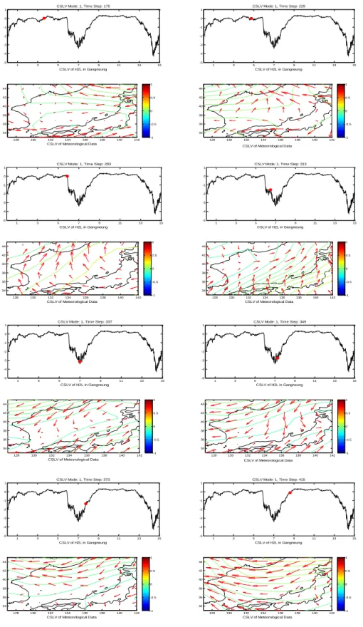
Next, to find the generation mechanism of sudden high waves, the evolution of spatial patterns of wind velocity and sea level pressures was presented during the sudden high wave events by CSEOF analysis and regression analysis. The wave data in Gangneung and Wangdolcho were used and the meteorological data were reanalysis data of National Centers for Environmental Prediction and National Center for Atmospheric Research (NCEP/NCAR). There are two peaks in the modes of all CSLV considered the physical process of sudden high waves. The patterns were categorized two groups. The first pattern was that the first peak was generated by low pressure moving to the north east part of the East Sea and easterly wind blowing for 1 day, whereas the second peak was caused by strong wind. The second pattern was that the first peak was affected by the wind speed in the east coast and the second peak was influenced by wind in the offshore area.

To forecast significant waves in multiple locations simultaneously, an EOFWNN model was developed by combining the EOF analysis and wavelet analysis with the neural network. The wave data used in this research were measured at eight wave observation stations in the East Sea and the meteorological

data were the NCEP/NCAR reanalysis data. The results of the EOFWNN model for significant wave height were compared with those of a wavelet and neural network hybrid (WNN) model in Gangneung, Sakata and Aomori for several lead times.

The EOFWNN model is better than the WNN model in that the former shows higher accuracy for longer lead times regardless of the wavelet decomposition level.

Significant wave period series were also forecasted using the EOFWNN model.

The results of significant wave period also show quite high accuracy. Also, the proposed model was employed to the numerical wave modeling data in the entire area of the East Sea. The results also show relatively high accuracy for one and three hour lead times.

Using the proposed intensity parameter of sudden high waves and the forecasted significant waves by the EOFWNN model, sudden high wave was detected and forecasted. From the forecasted wave data at 24 hour lead time,



^{H L2}



^{/ t}

  was calculated in Gangneung and Sakata. Although there is a slight deviation between the results of observed and forecasted wave data, sudden high wave was detected clearly.

Keywords: Artificial neural network; Empirical orthogonal function; Significant wave; Sudden high wave; Wave forecasting; Wavelet.

Student number: 2012-30953

TABLE OF CONTENTS

ABSTRACT ... i

LIST OF FIGURES ... vi

LIST OF TABLES ... xiv

LIST OF SYMBOLS ... xvi

CHAPTER 1 INTRODUCTION ... 1

1.1 Background ... 1

1.2 Research objectives ... 6

CHAPTER 2 THEORETICAL STUDY ... 8

2.1 Analysis methods of mechanism of sudden high waves ... 8

2.1.1 CSEOF analysis ... 9

2.1.2 Regreggion analysis ... 11

2.2 Wave forecast methods ... 13

2.2.1 EOF analysis ... 14

2.2.2 Wavelet analysis ... 16

2.2.3 Artificial Neural Network ... 19

2.2.4 EOF-Wavelet-ANN (EOFWNN) model ... 23

CHAPTER 3 CHARACTERISTICS OF SUDDEN HIGH WAVES ... 27

3.1 Data for anlaysis of characteristics of sudden high waves ... ... 27

3.1.1 Wave data ... 27

3.1.2 Meteorological data ... 27

3.3 Mechanism of sudden high waves ... 43

CHAPTER 4 FORECASTING OF SUDDEN HIGH WAVES .... 62

4.1 Data for forecasting of sudden high waves... 62

4.1.1 Observed wave data ... 62

4.1.2 Numerical wave modeling data ... 64

4.1.3 Meteorological data for forecasting ... 66

4.2 Forecasting of significant wave height and period using the observed data ... 67

4.3 Forecasting of significant wave height and peak period using the numerical modeling data ... 92

4.4 Detecting and forecasting of sudden high waves ... 103

CHAPTER 5 CONCLUSIONS ... 111

5.1 Summary and conclusions ... 111

5.2 Future study ... 114

REFERENCES ... 117

APPENDIX ... 121

국문초록 ... 137

LIST OF FIGURES

Fig. 1.1 Schematic diagram of the study ... 7

Fig. 2.1 ANN structure... 22

Fig. 2.2 Schematic diagram of the EOFWNN model ... 24

Fig. 2.3 Predictor configuration of wave forecasting model ... 26

Fig. 3.1 Wave measurement locations by KIOST ... 29

Fig. 3.2 Region of meteorological data ... 29

Fig. 3.3 Event of sudden high waves in October 2005 in Gangneung and Wangdolcho ... 31

Fig. 3.4 Illustration of high wave events ... 33

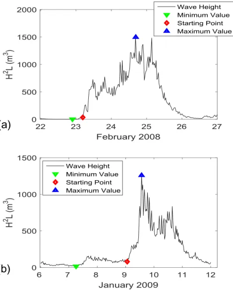
Fig. 3.5 Illustration of calculation of intensity parameter of sudden high waves in Gangnueng: (a) High wave event in February 23-25, 2008; and (b) High wave event in January 9- 11, 2009 ... 35

Fig. 3.6 Cumulative percentage curve of

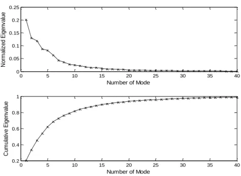
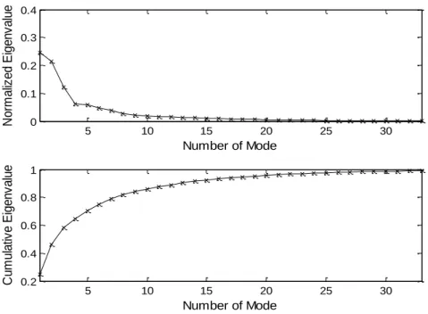
∆(𝐻²𝐿)/∆𝑡 ... 38

Fig. 3.7 Eigenvalues of CSEOF modes for significant wave height data from KIOST ... 44

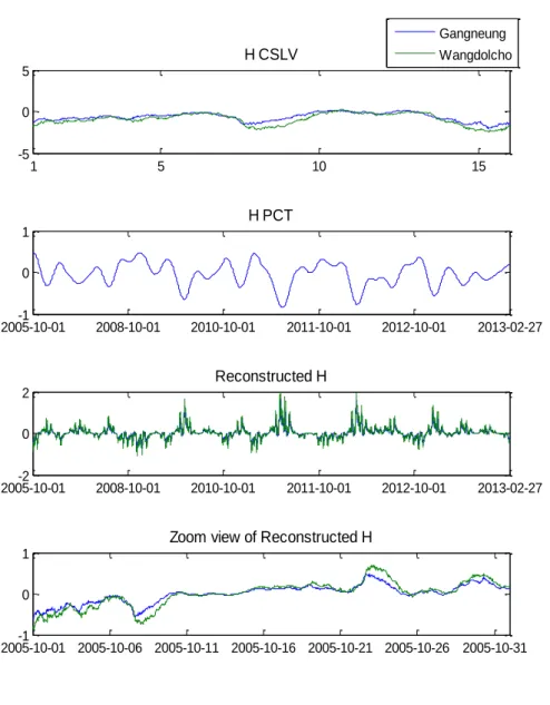
Fig. 3.8 CSEOF mode 1 of significant wave height data from

KIOST ... 45

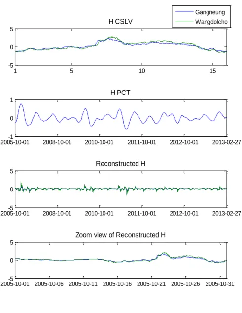
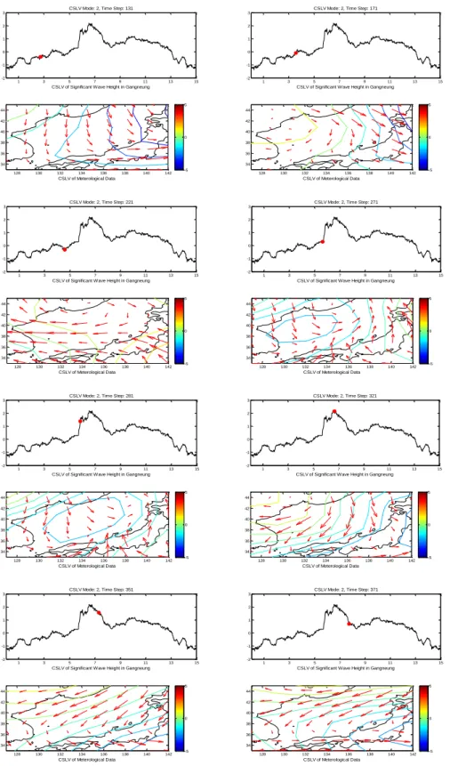
Fig. 3.9 CSEOF mode 2 of significant wave height data from

KIOST ... 46

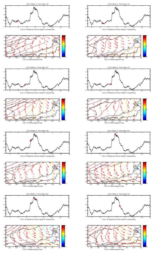
Fig. 3.10 CSEOF mode 3 of significant wave height data from KIOST ... 47

Fig. 3.11 Eigenvalues of CSEOF modes for sudden high wave index ... 48

Fig. 3.12 CSEOF mode 1 of sudden high wave index... 49

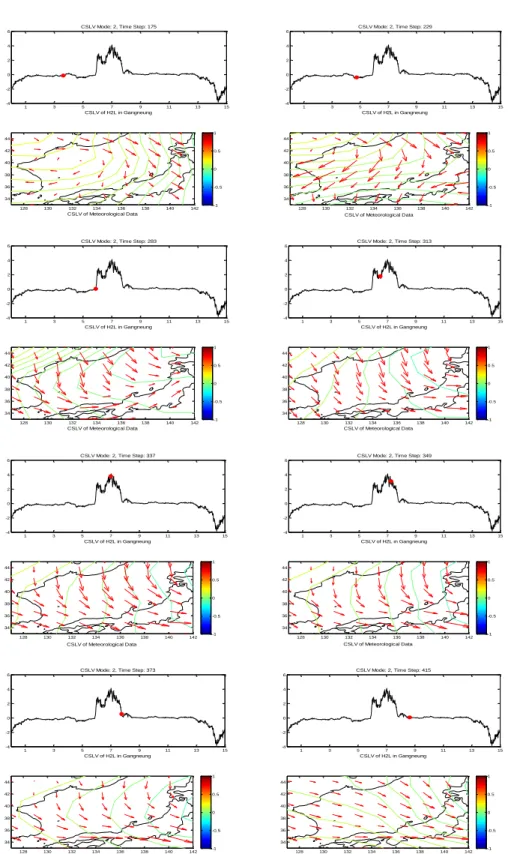
Fig. 3.13 CSEOF mode 2 of sudden high wave index... 50

Fig. 3.14 CSEOF mode 3 of sudden high wave index... 51

Fig. 3.15 Comparison of the first 2 modes of the regressed sea lavel pressure PC time series and significant wave height PC time series ... 53

Fig. 3.16 Comparison of the first 2 modes of the regressed wind speed PC time series and significant wave height PC time series ... 54

Fig. 3.17 Evolution of spatial patterns for the 2

^nd

mode of significant wave height and meteorological variables ... 56

Fig. 3.18 Evolution of spatial patterns for the 3

^rd

mode of

significant wave height and meteorological variables ... 57

Fig. 3.19 Comparision of the first 2 modes of the regressed sea level pressure PC time series and sudden high wave index PC

time series ... 58

Fig. 3.20 Comparision of the first 2 modes of the regressed wind speed PC time series and sudden high wave index PC time series ... 59

Fig. 3.21 Evolution of spatial patterns for the 1

^st

mode of sudden high wave index and meteorological variables ... 60

Fig. 3.22 Evolution of spatial patterns for the 2

^nd

mode of sudden high wave index and meteorological variables ... 61

Fig. 4.1 Wave measurement locations ... 63

Fig. 4.2 Grid map of KORDI (2005) ... 65

Fig. 4.3 Grid map of numerical wave modeling data ... 65

Fig. 4.4 First to fourth mode eigenvectors for wind velocity ... 68

Fig. 4.5 First to fourth mode eigenvectors for sea level pressure ... ... 68

Fig. 4.6 First to fourth mode PC time series for wind velocity .... 69

Fig. 4.7 First to fourth mode PC time series for sea level pressure .. ... 69

Fig. 4.8 Eigenvalues of EOF modes for significant wave height

data ... 70

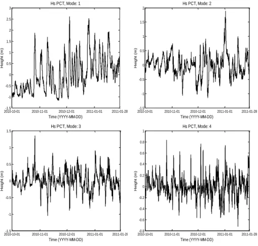
Fig. 4.9 First to fourth mode PC time series for significant wave height ... 71

Fig. 4.10 Decomposed wavelet components of the 1

^st

mode of H PC time series ... 72

Fig. 4.11 Approximations of the 1

^st

mode of wind speed and sea level pressure PC time series ... 72

Fig. 4.12 Largest R case for training period (Oct. 02, 2010 - Jan.

28, 2011) and ensemble members (black) and ensemble average (red) (00:00:00, Jan. 29, 2011) for the 1

^st

mode H PC time series for 1 hour lead time forecasting... 74

Fig. 4.13 Largest R case for training period (Oct. 02, 2010 - Jan.

27, 2011) and ensemble members (black) and ensemble average (red) (00:00:00, Jan. 29, 2011) for the 1

^st

mode H PC time series for 3 hour lead time forecasting... 74

Fig. 4.14 Largest R case for training period (Oct. 02, 2010 - Jan.

27, 2011) and ensemble members (black) and ensemble average (red) (00:00:00, Jan. 29, 2011) for the 1

^st

mode H PC time series for 12 hour lead time forecasting... 75

Fig. 4.15 Largest R case for training period (Oct. 02, 2010 - Jan.

27, 2011) and ensemble members (black) and ensemble

average (red) (00:00:00, Jan. 29, 2011) for the 1

^st

mode H PC

time series for 24 hour lead time forecasting... 75

Fig. 4.16 Comparison of observed (black circle) and estimated (blue triangle) wave height at 8 stations at 00:00:00, Jan. 29, 2011 (a) for 1 hour lead time, (b) for 3 hour lead time, (c) for 12 hour lead time, (d) for 24 hour lead time forecasting ... 76

Fig. 4.17 Observed and forecasted significant wave heights by WNN and EOFWNN models with 7

^th

decomposition level at 24 hour lead time in Gangneung ... 84

Fig. 4.18 Observed and forecasted significant wave heights by WNN and EOFWNN models with 7

^th

decomposition level at 24 hour lead time in Sakata ... 84

Fig. 4.19 Observed and forecasted significant wave heights by WNN and EOFWNN models with 7

^th

decomposition level at 24 hour lead time in Aomori ... 85

Fig. 4.20 Comparison of index of agreement between EOFWNN and WNN model with 3, 5, and 7 decomposition level in several lead times in (a) Gangneung, (b) Sakata, (c) Aomori ...

... 86

Fig. 4.21 First to fourth mode PC time series for significant wave period ... 88

Fig. 4.22 Observed and forecasted significant wave period by

EOFWNN model with 7

^th

decomposition level at 24 hour

lead time in Gangneung ... 90

Fig. 4.23 Observed and forecasted significant wave period by EOFWNN model with 7

^th

dedomposition level at 24 hour lead time in Sakata ... 90

Fig. 4.24 Observed and forecasted significant wave period by EOFWNN model with 7

^th

dedomposition level at 24 hour lead time in Aomori ... 91

Fig. 4.25 First four modes of eigenvectors for wind velocity ... 93

Fig. 4.26 First four modes of PC time series for wind velocity ... 93

Fig. 4.27 First mode of eigenvector and corresponding PC time series of significant wave height for numerical wave modeling data... 94

Fig. 4.28 Coefficient of correlation of EOFWNN model for numerical results of significant wave height with 7

^th

decomposition level at 3 hr lead time ... 95

Fig. 4.29 Index of agreement of EOFWNN model for numerical results of significant wave height with 7

^th

decomposition level at 3 hr lead time... 96

Fig. 4.30 NRMSE of EOFWNN model for numerical results of significant wave height with 7

^th

decomposition level at 3 hr lead time... 96

Fig. 4.31 Highest performance case of EOFWNN model for

numerical results of significant wave height with 7

^th

decomposition level at 3 hr lead time ... 97

Fig. 4.32 Lowest performance case of EOFWNN model for numerical results of significant wave height with 7

^th

decomposition level at 3 hr lead time ... 97

Fig. 4.33 Firtst mode of the eigenvector and corresponding PC time series of peak period for numerical wave modeling data ...

... 99

Fig. 4.34 Coefficient of correlation of EOFWNN model for numerical results of peak period with 7

^th

decomposition level at 3 hr lead time ... 100

Fig. 4.35 Index of agreement of EOFWNN model for numerical results of peak period with 7

^th

decomposition level at 3 hr lead time... 100

Fig. 4.36 NRMSE of EOFWNN model for numerical results of peak period with 7

^th

decomposition level at 3 hr lead time .. 101

Fig. 4.37 Highest performance case of EOFWNN model for numerical results of peak period with 7

^th

decomposition level at 3 hr lead time ... 101

Fig. 4.38 Lowest performance case of EOFWNN model for numerical results of peak period with 7

^th

decomposition level at 3 hr lead time ... 102

Fig. 4.39 Snapshots of



( H L

²

) /



t calculated during the period

of February 2-3, 1987: (a) 9am Feb. 2

^nd

(b) 1am Feb. 3

^rd

(c) 6am Feb. 3

^rd

(d) 2pm Feb. 3

^rd

... 104

Fig. 4.40 Locations of wave observation stations of NOWPHAS system ... 105

Fig. 4.41 Temporal variation of H L

²

measured at three wave stations of NOWPHAS system in Februaru 1-5, 1987: (a) Hamada (b)Tottori and (c) Ka azawa ... 107

Fig. 4.42 Comparison of Temporal variation of H L

²

between observed and forecasted wave data at 24 hour lead time in Gangneung ... 109

Fig. 4.43 Comparison of Temporal variation of H L

²

between observed and forecasted wave data at 24 hour lead time in Sakata ... 110

Fig. 5.1 Autocorrelation of residuals of observed and forecasted

results for significant wave height at 24 hour lead time in

Gangneung ... 116

LIST OF TABLES

Table 3.1 Marine accidents and/or property damage along the coast of Gangwon-do Province and Gyeongsangbuk-do Province (from Geosystem Research, 2015) ... 37

Table 3.2 Characteristics of

∆𝐻/∆𝑡

and

∆(𝐻²𝐿)/∆𝑡

in Gangneung ... 38

Table 3.3 Comparison of sudden high wave events of

∆(𝐻²𝐿)/

∆𝑡 ≥ 80 m³/hr and marine accidents ... 40

Table 3.4 Precipitation and maximum wind speed during marine accident and/or property damage due to sudden high waves ...

... 42

Table 4.1 Information on wave measurement stations and statistical properties of wave data at each station ... 63

Table 4.2 Test results of WNN model for H in Gangneung, Sakata and Aomori for several lead times ... 78

Table 4.3 Test results of EOFWNN model for H at 1 hr lead time depending on decoposition level ... 80

Table 4.4 Test results of EOFWNN model for H at 3 hr lead time depending on decoposition level ... 81

Table 4.5 Test results of EOFWNN model for H at 12 hr lead

Table 4.6 Test results of EOFWNN model for H at 24 hr lead time depending on decoposition level ... 83

Table 4.7 Test results of EOFWNN model for T at 8 stations for several lead times with decomposition level 7 ... 89

Table 4.8 Disaster damage occurred in February 3-4, 1987, in

Shimane Prefecture, Japan (unit = 1,000 Japanese Yen) ... 105

LIST OF SYMBOLS

Comprehensive Explanations

 Unless otherwise stated, all the wave parameters are those of significant waves (e.g. H = significant wave height).

Latin Uppercase A: approximation 𝐵_𝑛(𝑥): eigenfunction

𝐵_𝑛(𝑥, 𝑡), 𝐶_𝑛(x, 𝑡), 𝐷_𝑛(x, 𝑡): cyclo-stationary loading vector (CSLV) D: detail

H: wave height (m) 𝐼_𝑎: index of agreement

L: wave length (m)

NRMSE: normalized root mean square error R: correlation coefficient

RMSE: root mean square error T : wave period (s)

T (x,t), P (x,t): spatio-temporal series

𝑇_𝑛(𝑡), 𝑃_𝑛(𝑡): principal component (PC) time series

Latin Lowercase a: scale factor

b: shift factor or ANN bias

d: nested period

slp: sea level pressure series t, 𝑡^′: time

w: ANN weight

wnd: wind velocity series x, 𝑥^′: space

Greek Lowercase

α_𝑚^{𝑛}: regression coefficient

ε^{𝑛}(𝑡): regression error time series 𝜆_𝑛: eigenvalue

𝜙: scaling function 𝜓_𝑛: wavelet function

CHAPTER 1. INTRODUCTION

1.1 Background

Recently, exceptional high waves have caused many casualties and serious property damage in the East Sea of Korea. On 21 October 2006, the significant wave height reached 9.69 m and its peak period was 12.8 s near Sokcho Harbor, which was the maximum wave height ever observed on the east coast of Korea (Jeong, Oh, and Lee 2007). Meanwhile, similar events have been repeatedly reported on the west coast of Japan. Many researchers examined the most remarkable event occurred on 24 February 2008 at Toyama Bay, which was highlighted by the significant wave height of 9.92 m (Mase et al. 2008, Lee et al.

2010). These disastrous waves claimed the losses of life more than 50 people during the ten years between 2005 and 2015 in the east coast of Korea because they suddenly occurred under the relatively mild weather in the winter season.

Although storm waves about two times higher than 50 year return period of deep water design waves have been observed in the east coast, sudden high waves have not been considered until now when estimating design waves of coastal structures. The high waves occur repeatedly every year and the risk of sudden high waves will increase due to anomaly climate such as global warming, so it is necessary to take into account such high waves when estimating design waves (Jeong, Oh, and Lee 2007). Since figuring out sudden high waves is the key factor not only in coastal damage and disaster but also in the design of coastal structures, it is critical to forecast sudden high waves accurately.

long ago (Kitaide 1952, Isozaki 1971, Isozaki and Yoshio 1972). Recently, as casualties and property damage caused by sudden high waves have been increased, researches have been made actively (Jeong 2009, Lee et al. 2010, Oh et al. 2010, Kashima and Hirayama 2011, Ahn et al. 2013, Oh and Jeong 2013, Lee et al. 2014).

The studies are divided into two major parts: analysis of the characteristics and mechanism of sudden high waves and forecasting of sudden high waves using numerical method.

Definition of sudden high waves

Kim and Lee (2008b) analyzed the observed swells in Wangdolcho on 22 – 28 February 2008 using wavelet method. They showed that the peak frequency moves to the lower frequency and the wave energy increases dramatically during the event.

Oh et al. (2010) analyzed several events and described the causes of high waves for each case. They defined such high wave as large-height swell-like wave, which often has a larger height than general swell (H > 3 m) and a relatively long period (T > 9 s). Since their research, many researchers have followed their definition of large-height swell-like waves. Also, the many have classified such waves according to only its height and period. However, the definition and criteria of the high waves is vague and insufficient because the high waves have the characteristics of both swell and wind wave and the definition does not reflect the rapid increase of waves in a few hours. In this study, sudden high wave was used as a new terminology to include the characteristics of such high waves.

Generation mechanism of sudden high waves

The mechanism of sudden high waves have been analyzed not only in the field of coastal engineering but also meteorology. According to Kitaide (1952), the waves called “Yorimawari wave” in Japan are generated due to the strong north

and northeasterly winds formed by a quasi-stationary developed atmospheric low- pressure area. Isozaki (1971) and Isozaki and Yoshio (1972) examined the characteristics of abnormal high waves and described the predictability based on meteorological observations of past events. Joung et al. (1984) studied the generation process of a low-pressure system developed on 2 January 1981 by using the results from an adiabatic inviscid quasi-geostrophic model. Jeong, Oh, and Lee (2007) analyzed the characteristics of the high waves observed at 5 stations in the East Sea on 23–24 October 2006 with wind data. According to them, sudden high waves occurs due to superposition of wind waves and swell generated by strong East Sea twister. Oh and Jeong (2013) analyzed the characteristics of sudden high waves and meteorological conditions during the events using the observed wave data at multiple stations along the east coast of Korea. According to them, important is not only the pressure drop during the movement of low pressure system but also other factors such as moving trajectory and staying time of the low pressure system together with arrangement of neighboring atmospheric pressure fields. They also found that the spectral density of the high waves increases two times on 23 February 2008. It was found that the characteristics of waves would be predominantly governed by long-traveled swell in the former case but in contrast, it would be a result of local wind sea development in the latter case. Although many researches related to generation mechanism of sudden high waves have been studied, they are only for a few cases based on casualties or damage of properties.

It is necessary to analyze the overall generation mechanism of sudden high waves using the wave data measured long period.

Forecasting of sudden high waves

have been conducted (Ahn et al. 2013, Hatada and Yamaguchi 1998, Kim and Lee 2008a, Kim et al. 2011, Lee et al. 2008, Lee et al. 2014, Mase et al. 2008). Even though many researches for forecasting of sudden high waves have been done, they have been studied only using numerical methods. There is no research for forecasting of sudden high waves using statistical method such as machine-learning until now.

Machine-learning forecasting of significant wave heights

Despite of considerable advances in computational techniques, the solutions obtained by numerically solving the equations of wave growth are neither exact nor uniformly applicable at all sites and at all times due to the complexity and uncertainty of the wave generation phenomenon (Deo et al. 2001). Prediction of waves is basically uncertain and random process and hence difficult to model by using deterministic equations. Therefore, many researchers have established the forecasting of waves using stochastic models such as auto-regressive moving average (ARMA), auto-regressive integrated moving average (ARIMA) or artificial neural networks (ANN).

Deo et al. (2001) explored the possibility of employing neural networks for weakly mean wave forecasting based on wind speeds. They mentioned that neural network modeling is proper to predict waves since it is primarily aimed at recognition of a random pattern in a given set of input values and does not require knowledge of the physical process as a precondition. However, their results are not very satisfactory, possibly due to the uncertainties of the wind-wave relationship.

After their research, many researchers have investigated wave forecasting using artificial neural network by training the observed wave records directly (Tsai, Lin, and Shen 2002, Makarynskyy et al. 2005, Londhe and Panchang 2006). Their

results showed the short-term forecasts (3 and 6 hours) of the wave parameters are more accurate than longer-term forecasts. Meanwhile, some researchers have examined the effects of other meteorological factors on wave height forecasting using ANN (Günaydın 2008, Zamani et al. 2008). However, there is no significant improvement of the forecasting results.

Even though ANN has flexibility, it may not be able to cope with non- stationary data without any preprocessing of the input and output data (Cannas et al.

2006). In the recent years, hybridization of ANN with other techniques has been used in wave height forecasting to provide effective modeling. Ö zger (2010) proposed the combination of wavelet and fuzzy logic approaches to forecast wave height up to 48 hour lead time. Deka and Prahlada (2012), Prahlada and Deka (2015) used wavelet neural network (WNN) for wave height forecasting up to 48 hour lead time. Dixit and Londhe (2016) also used neuro wavelet technique for extreme wave heights forecasting up to 36 hour lead time. Shahabi, Khanjani, and Kermani (2016) developed genetic programming based wavelet transform to forecast significant wave height up to 48 hour lead time. Hybrid model results showed better prediction performance than single ANN model. Although their results indicates good predictions at lower lead times but slight deviation is observed at higher lead times. Also there are limitations that their models cannot interpret the relationship between spatially distributed meteorological variables and waves and cannot forecast spatially distributed wave height at once. In other words, in their researches modeling is performed for forecasting wave height at different locations separately.

1.2 Research Objectives

The ultimate goal of this study is to forecast sudden high waves in the East Sea of Korea based on the meteorological data and wave data using machine-learning. To forecast the waves, the first objective is to define a new intensity parameter of sudden high waves. Second, the generation mechanism of the waves are investigated by analyzing the relation between waves and meteorological variables.

Third, significant wave height and period are forecasted in the East Sea of Korea using machine-learning. Finally, sudden high waves are detected and forecasted from the proposed intensity parameter and the forecasted significant waves in the East Sea of Korea. Fig. 1.1 shows the schematic diagram of this study.

This thesis is organized in the following order. Chapter 2 explains the statistical methods to analyze and forecast sudden high waves. Chapter 3 consists of three parts; (1) description of data (2) definition of sudden high waves and (3) generation mechanism of sudden high waves. Chapter 4 consists of four parts; (1) description of data (2) forecasting of the significant wave height and period using the observed data along the coast of the East Sea, (3) forecasting of the significant wave height and period using the numerical modeling data in the entire area of the East Sea and (4) detection and forecast of sudden high waves. In Chapter 5, the conclusions are given and future work is discussed.

Fig. 1.1 Schematic diagram of the study

CHAPTER 2. THEORETICAL STUDY

2.1 Analysis methods of mechanism of sudden high waves

Some geophysical and climatic variables have periodically time-dependent covariance statistics or non-stationarity. Stationarity assumption is often not appropriate for such geophysical and climate variables even after removing the diurnal cycle or the seasonal cycle (Kim, Hamlington, and Na 2015). A proper recognition of the time-dependent response characteristics is vital in accurately extracting physically meaningful modes and their space-time evolutions from data.

Cyclostationary empirical orthogonal function (CSEOF) analysis is an alternative to regular EOF analysis or other eigen-analysis techniques based on the stationarity assumption to extract physical modes. In this study, the CSEOF analysis was used to examine the physical processes of sudden high waves. When a physical process undergoes a stochastic variation for some reasons, two physical variables describing the process evolve in the same fashion (Kim, Hamlington, and Na 2015).

If the system is linear, their relationship may be linear. However, due to the complexity of the system, it is difficult to find the relationship between the physical variables directly. Therefore, a proper distinction from stochastic undulation and explanation of time-dependent physical response are vital in accurately determining physically consistent or teleconnection response in different variables.

This can be achieved by the regression analysis in CSEOF space (Kim and Chung 2001, Seo and Kim 2003, Hamlington et al. 2011, Kim, Hamlington, and Na 2015).

2.1.1 CSEOF analysis

Kim, North, and Huang (1996) and Kim and North (1997) introduced the concept of CSEOF analysis to capture the time-varying spatial patterns and longer-time- scale fluctuations in geophysical data. The difference between EOF analysis and CSEOF analysis is the ability of CSEOF analysis to extract spatial patterns varying in time and space. This is possible because the CSEOF spatial patterns are time dependent, whereas EOF spatial patterns are only varying spatially (Strassburg et al.

2014).

In a CSEOF analysis, space-time data are decomposed into:

( , ) = _{n n}( , ) ( )_n

T x t



B x t T t , (2.1)

where B x t_n( , )B x t_n( , d) are the CSEOF loading vectors (CSLV), which are multiple (d) spatial patterns and repeat themselves in time and T tn( ) are the corresponding principal component (PC) time series (Kim, North, and Huang 1996, Kim and North 1997). In other words, B x t_n( , )are time-dependent physics and

n( )

T t are the stochastic undulation of the physical processes. The CSLVs and the corresponding PC time series are obtained by solving:



^{, ; ,' '}



n^{( , )' '} n n^{( , )}

C x t x t B x t  B x t , (2.2)

with xand x^'representing different points in space and time, respectively. The

space-time covariance function is periodic in time with the nested period d.



^{, ; ,' '}

 

^{, ; ,' '}



^.

C x t x t C x td x t d (2.3)

Since the covariance matrix cannot be written as a square matrix, Eq. (2.2) cannot be solved in the same manner as EOF analysis. Instead, it can be solved by taking Fourier transform twice with respect to t and t^', making use of the assumption that the covariance matrix is periodic. The PC time series in Fourier space are easy to obtain, and then both the CSLVs and PC time series are transformed back to physical space (Kim, North, and Huang 1996, Hamlington et al. 2011).

While the assumption of periodic statistics may be reasonable for many geophysical variables, it is difficult to prove the periodicity of statistics and identify the period. The periodicity is called “nested period”. The nested period is often determined based on a priori physical understanding of the physical process to be investigated (Kim, Hamlington, and Na 2015). However, sometimes the period of a physical process is not obvious mainly because of the lack of understanding of the underlying physical process. It is also difficult to find the nested period because multiple physical processes have different periods. Let us consider a dataset consisting of several physical processes

( , ) ( , )

n n n

B x t B x td (2.4)

where d_nis the period of a physical process B x t_n( , ). If it is assumed that the PC time series, T t_n( ), are stationary, then the first two moment statistics are:

   

 

 

, , ( , ) ( )

( , ) ( ) ,

,

n n

n

n n

n

x t T x t B x t T t

B x t d T t d T x t d x t d





 

    

 





(2.5)

         

   

     

' ' ' ' ' ' '

' ' '

' ' ' '

, ; , , , ( , ) , ( )

= ( , ) , ( )

, , , ; ,

n n n m

n m

n n n m

n m

C x t x t T x t T x t B x t B x t T t T t B x t d B x t d T t d T t d T x t d T x t d C x t d x t d

 

   

     

 

 

(2.6)

if d is given as the least common multiple of

 

dn , i.e., dLCM d

 

n . Under the assumption of stationarity of PC time series, the first two moment statistics are functions of time lag tt^'. Thus, the period of the first two moment statistics of a given dataset is the least common multiple of all physical periods in the dataset.

The consequence of the nested period being the least common multiple of all physical periods is that physical processes with period less than d are shown to repeat in CSLVs. Although the nested period can be set to be an integral multiple of least common multiple of all physical periods, the minimum period should be used in order to minimize the contamination of covariance statistics by sampling errors (Kim, Hamlington, and Na 2015).

2.1.2 Regression analysis

First, the CSEOF analysis is conducted on a target variable (wave height and wave period) and predictor variable (meteorological data):

- Target variable:

( , ) = _{n n}( , ) ( )_n

T x t



B x t T t (2.7 a) - Predictor variable:

( , ) = _{m m}( , ) _m( )

P x t



C x t P t (2.7 b)

where B x t_n( , ) and C_m( , )x t are the CSLVs of the target and predictor variables, respectively, and T t_n( ) and P t_m( ) are the PC time series of the target and predictor time series, respectively. Then, conducting regression analysis between the two PC time series gives:

 

^M₁ ^{ n}

 

^{ n}

 

, 1, 2,

n m m m

T t 



_ a P t  t n (2.8)

where

 

^{am n} are the regression coefficients, ^{ n}

 

^t is the regression error time series, and M is the number of predictor time series modes used in the regression.

The regression coefficients are determined so that the variance of regression error is minimized. Using the regression coefficient, the evolution of the predictor variable, which is physically consistent with the target evolution, is obtained:

 

^{, M}₁ ^{ n}

 

^,

n m m m

D x t 



_ a C r t (2.9)

where Cm

 

x t^, is the CSLV of predictor variable and D x tn

 

^, is the consistent CSLV with the target variable. In this way, the evolution of any variables can be achieved to be physically consistent with that of the target variable. The consistent patterns of two physical variables may not generally have the same physical

response characteristics. However, the physical relationship between physically consistent patterns of two or more physical variables should be dictated by a governing equation describing the particular physical process they represent. It is the stochastic component of undulation that should be identical in the evolution of two physical variables originating from the same physical process (Kim, Hamlington, and Na 2015).

2.2 Wave forecast methods

Prediction of waves is basically uncertain and random process and hence difficult to model by using deterministic equations. Artificial neural network (ANN) is suitable for partially understood underlying physical processes such as wind-wave relationship. In spite of suitable flexibility of ANN, it may not be able to cope with non-stationary data if pre-processing of the input and output data is not performed (Cannas et al. 2006). Also it is difficult to interpret the relationship between spatially distributed meteorological variables and waves. Principal component analysis (PCA), also called the empirical orthogonal function (EOF) analysis is a useful tool to interpret physical processes in the data. The assumption in the EOF analysis is the stationarity of the data. It means that the covariance function of the data does not depend on time. As I mentioned in previous section, the stationarity assumption is often not appropriate for such geophysical and climate variables. In previous section, CSEOF analysis was suggested as an alternative to EOF analysis to extract physical modes. However, to forecast wave series, spatial components and temporal components should be separated completely. Thus, in this section,

EOF analysis is introduced to interpret the relationship between waves and meteorological data. Also, EOF analysis make the proposed model to forecast wave data at multi-stations simultaneously. To overcome stationarity assumption of the EOF analysis, wavelet analysis is combined. Wavelet analysis can handle non- stationary and transient signals as well as fractal-type structure (Murguia and Campos-Cantón 2006). In this study, a hybrid empirical orthogonal function analysis (EOF)–wavelet analysis–ANN (EOFWNN) model is introduced and employed to forecast significant wave height (or period). The decomposed time series are used as inputs to ANN which can handle non-stationarity and non- linearity efficiently.

2.2.1 EOF analysis

EOF analysis, also known as the principal component analysis, or singular value decomposition method, can be utilized effectively to link the spatial and temporal patterns of a data field (Legler 1983). This method partitions the temporal variance of the data into orthogonal spatial patterns called eigenvectors.

Space-time data can be decomposed in terms of EOFs. That is,

 

, _n

   

_n

n

T x t 



T t B x ^(2.10)

where



B xn

  

are called eigenfunctions and



T tn

  

are expansion of coefficients that are functions of time. Eq. (2.10) is called EOF decomposition only

if



B xn

  

are mutually orthogonal to each other and



T tn

  

are mutually uncorrelated. That is,

       

1

1 ^N

n m n m nm

x

B x B x B x B x

N 



 



 (2.11)

       

1

1 ^N

n m n m n nm

t

T t T t T t T t

N  



 



 (2.12)

where _nmis Kronecker delta and _nis eigenvalues. Often,



B xn

  

are called loading vectors,



T tn

  

principal component (PC) time series. Spatial covariance function defines covriance between two spatial points x and x’:



^{, '}

    

^{, ',}

C x x  T x t T x t (2.13)

which under the stationarity aussumption can be written as

     

1

, ' 1 , ',

N t

C x x T x t T x t N 





(2.14)

In terms of EOFs, spatial covariance matrix is

         

       

   

, ' '

'

'

n n m m

n m

n m n m

n m

C x x T t B x T t B x B x B x T t T t B x B x









 





(2.15)

Dot product of Eq. (2.15) with Bm

 

x^' yields

         

   

, ' ' ' '

m n n n m

n

n n nm m m

n

C x x B x B x B x B x

B x B x



  

  

 





(2.16)

It is called the Karhunen-Loѐvé equation. It is similar to the eigenvalue problem (Kim, Hamlington, and Na 2015).

2.2.2 Wavelet analysis

Wavelet analysis (WA), which provides a perfect filtering characteristic, has been used in various fields of mathematics, science, and engineering. Through the decomposition and reconstruction of a signal, WA can be performed to determine the transient identity in the time-frequency domain (Wang, Lee, and Zhang 2004).

Unlike Fourier technique or EOF analysis, the basis function of the wavelet transform has the key property of localization in time (or space) and frequency.

This makes the wavelets ideal for handling non-stationary and transient signals, as well as fractal-type structures (Murguia and Campos-Cantón 2006).

Wavelet analysis is used to decompose or reconstruct a signal using the wavelet functions. The wavelets are a family of orthogonal functions of type,

 

1/2

, ( ) ( ) / , , , 0

a b t a t b a a b R a

  ^     (2.17)

generated from a “mother” wavelet function ( )t by dilation and translation

operations, which are governed by the scale factor a and shift factor b , respectively.

The continuous wavelet transform (CWT) and its reconstruction version of a signal f t( )L R²( ) are defines as,

W a b_f( , ) a^{1/ 2 } f t( )^*



(t b) /a dt



f t( ), _{a b}, ( )t





    (2.18)

1 2

( ) _f( , ) _{a b}, ( ) /

f t C_{  }^

 

^{ }W a b t a dadb (2.19)

where, ^*



^{(tb) /a}



^{is the complex conjugate of }



^{(tb) /a}



^,

2

( ) / , ( )

C_ 



_^ F_   d F_  is the Fourier transform of ( )t .

To avoid the redundancy in CWT, a so-called dyadic discrete wavelet transform DWT, is usually adopted in engineering practice. Letting a2 ,^j

2 ^j

b ^ k ( ,j kZ), Eq. (3.18) and (3.19) may be rewritten in a dyadic discrete form,

𝑊_𝑓(𝑎, 𝑏) = 𝑊_𝑓(2^𝑗, 2^−𝑗𝑘) = 2^𝑗∫ 𝜓(2_−∞^{∞ 𝑗}𝑡 − 𝑘)𝑓(𝑡)𝑑𝑡 (2.20) ( ) _f(2 , 2^{j j} ) (2^j )

j k

f t 

 

W ^{ } k  tk (2.21)

The theory is referred to Wang et al. (2004).

In wavelet analysis, original series are decomposed into approximation and detail. The approximations are the high-scale, low-frequency components of the signal. The details are the low-scale, high-frequency components. The filtering process, at its most basic level, the original signal passes through two complementary filters and emerges as two signals. The selection of a suitable level for the hierarchy depends on the signal and experience. Often the level is chosen

based on a desired low-pass cutoff frequency.

In this process, the length of data becomes twice as much data as started. They are the signals A and D. To fix the extended length into the original length, downsampling is necessary. Through the process of downsampling, two sequences called cA and cD are achieved. After this process, DWT coefficients are produced.

The decomposition can be iterated, with successive approximations being decomposed in turn, so that one signal is broken down into many lower resolution components. This is called the wavelet decomposition tree.

The organizing parameter, the scale a, is related to level j by a2^j. If resolution is defined as 1/a, then the resolution increases as the scale decreases.

The greater the resolution, the smaller and finer are the details that can be accessed.

From a technical point of view, the size of the revealed details for any j is proportional to the size of the domain in which the wavelet or analyzing function of the variable ^{x, }



^{x a/}



is not too close to 0.

The process of reconstruction assembles the decomposed components back into the original signal without loss of information. The mathematical manipulation that produces this synthesis is called the inverse discrete wavelet transform (IDWT). Where wavelet analysis involves filtering and downsampling, the wavelet reconstruction process consists of upsampling and filtering. Upsampling is the process of lengthening a signal component by inserting zeros between samples.

The low- and high-pass decomposition filters (L and H), together with their associated reconstruction filters (L` and H`), form a system of what is called quadrature mirror filters.

There are several types of wavelet families such as Daubechies, Biorthogonal, Coiflets, Symlets, Morlet, etc. In this study, Coiflet5 (coif5) was used. This wavelet function  has 2N moments equal to 0 and the scaling function  has 2N-1 moments equal to 0. The two functions have a support of length 6N-1. The coifN

 and  are much more symmetrical than the dbNs (Daubechies). With respect

to the support length, coifN has to be compared to db3N or sym3N (Symlets), which belong to yet another wavelet family. The wavelet analysis was carried out using MATLAB toolbox.

2.2.3 Artificial Neural Network

Artificial neural network (ANN) is suitable for partially understood underlying physical processes such as wind-wave relationship. Fig. 2.1 shows the structure of feed forward back propagation type of ANN, which consists of an input layer, one or more hidden layers, and an output layer. These layers have one or more nodes.

The source nodes in the input layer propagate through the network in a forward direction. Each node of a layer connects that of the next layer. The back- propagation learning consists of two passes through the different layers of the network: a forward pass and a backward pass. In the forward pass, an input vector is applied to the sensory nodes of the network and its effect propagates through the network layer by layer. Finally, a set of outputs is produced as the actual response of the network. During the forward pass, all the synoptic weights of the networks are fixed. During the backward pass, on the other hand, all the synoptic weights are adjusted in accordance with an error correction rule (Günaydın 2008).

The outputs of the hidden layer are calculated from



^{1 1}



. _j ( _j) ⁿ_{i ij i} , 1, 2, ,

H O  f net  f



_ w IO b j n (2.22) where b₁ is the first layer bias, ^f

 

is the transfer function between input and

hidden layers. In the present study, a sigmoid transfer function of the type

 

^{j 1 / 1 exp}

 

^j

 

f net   net is used. Outputs of the output layer are determined as follows:



^{0 2}



. _k ( _k) ^h_j^m _jk . _j , 1

O O  f net  f



_ w H O b k (2.23)

where b₂ is the second layer bias, ^f

 

is the transfer function between hidden and output layers. In this study, a linear transfer function f net( _k)net_kis used.

To avoid the problem of overfitting that may occur while an ANN is being trained, the number of nodes in the hidden layer, z, of the nets employed in the first stages of the study was computed using one of the empirical expressions mentioned by Fletcher and Goss (1993)

2n1/ 2m (2.24)

where n is the number of input nodes and m is the number of output nodes.

In training schemes the difference or the error between the network-yielded and the target or actual output is minimized using a particular mathematical algorithm. The global (mean sum squared) error (E), is defined as follows:

 

²

1

1 .

2

l

p k k k

e 



_ T O O (2.25)

1

1 P

p p

E e

P ^





(2.26)

where T_k is the target (observed) output at the kth output node, O O. _k is the predicted output at the kth output node, P is total number of training patterns, and epis the error for the pth training pattern. The procedure of back propagation network is to propagate the error at the output layer backward from the output to hidden layer in order to adjust the weights in each layer of the network.

There are several training algorithms such as Resilient back-Propagation (RP), Scaled Conjugate Gradient (SCG), Conjugate Gradient Powell-Beale (CGB), Broyden, Fletcher, Goldfarb (BFG), and Levenberg-Marquardt (LM). The rate of change of error with respect to the connection weights, i.e. the error gradient is used as a path to do so. A general conjugate gradient scheme involves performing a search along the conjugate or orthogonal direction in order to determine the step size to minimize the performance function. Among the algorithms, the LM is the fastest method for training moderate-sized feedforward neural networks. However, it requires the storage of some matrices that can be quite large for certain problems.

In this research, the network is very large, so one of the conjugated gradient algorithms is recommended (Demuth and Beale 2000). Kalra et al. (2005) compared the prediction performance of the five algorithms and mentioned that the CGB produced the most accurate results among the algorithms. Therefore, the CGB scheme was used in this study. The ANN model implementation was carried out using MATLAB toolbox.

Fig. 2.1 ANN structure

2.2.4 EOF-Wavelet-ANN (EOFWNN) model

In this study, the combination of neural network, EOF analysis and wavelet analysis was employed to forecast significant wave height and period from observed wave data and reanalysis meteorological data. Fig. 2.2 is the schematic diagram of the EOFWNN model, which is the detailed flow chart of the right side of Fig. 1.1. First, EOF analysis was conducted for wave data and meteorological data to separate spatial and temporal components for training period. Second, wavelet analysis was applied to each PC time series of wave data and meteorological data. Next, training was conducted with the decomposed wavelet component time series of wind speed, sea level pressure and wave height (or period) data as input data and each PC time series of wave height (or period) data for various lead times for target. Finally, the forecasted wave height (or period) PC time series and the LVs obtained in the first step were reconstructed to calculate the wave height (or period) time series.

The decomposed wavelet signals of wave data and meteorological data used as the input to the ANN were those of all the decomposed PC time series of significant wave height and the approximations of 90% PC time series of meteorological data. To consider the dominance of persistence in the wave height time series, the significant wave heights at the present time and the previous two time steps were used as predictors. To consider the time lag effect of meteorological data, the meteorological data at the forecast lead time and at one and six time steps ahead of that time were used as predictors. In summary, the scenario formed by predictor configuration to predict H t(  n t) is H(t),

Fig. 2.2 Schematic diagram of the EOFWNN model

( )

H t t , H t(  2 t), wnd t(  n t), wnd t(    n t t), wnd t(    n t 6 t),

( )

slp t n t , slp t(    n t t), slp t(    n t 6 t). Where, H(t) is the wavelet component of the present wave height, H t(  t)and H t(  2 t) are previous time steps, H t(  n t) is the PC time series of significant wave height at the forecast lead time, wnd t(  n t)and slp t(  n t)are the wavelet components of wind speed and sea level pressure at the forecast lead time, and wnd t(    n t t),

( 6 )

wnd t   n t t , slp t(    n t t), slp t(    n t 6 t) are those at previous time steps from the forecast lead time, and ‘n t ’ denotes the forecast lead time.

The lead times were fixed as 1, 3, 12, and 24 hours with the use of  t 0.5 hr. The meteorological data at tand 6t ahead of the forecast lead time were arbitrarily chosen by supposing that the wave height at a certain time would be closely related to the meteorological conditions at 30 minutes and 3 hours ahead of the time. Fig. 2.3 shows the predictor configuration of wave forecasting model.

The performance was repeated 20 times, and then ensemble members were averaged. After removing the two cases of the largest root mean squared error (RMSE) between ensemble average and each member, the remaining 18 ensemble members were averaged.

Fig. 2.3 Predictor configuration of wave forecasting model

CHAPTER 3. CHARACTERISTICS OF SUDDEN HIGH WAVES

3.1 Data for analysis of characteristics of sudden high waves

3.1.1 Wave data

To examine the characteristics of sudden high waves that caused marine accidents and property damage, investigations were made into the wave data at Gangneung and Wangdolcho on the east coast of Korea. The wave data were provided by KIOST (Korea Institute of Ocean Science and Technology). Fig. 3.1 shows the locations of wave measurement. The wave data of KIOST was measured every 0.5 s using pressure gauge and sampling rate is ∆𝑓 ≈ 0.008 𝐻𝑧. Wave spectrum was calculated every 30 minutes from the collected wave series. The water depths at the wave measurement stations were 15.0 and 15.3 m, respectively. Experiments were conducted for the winter season from October to February, when sudden high waves occur frequently. The period is 5 years in 2005, 2008, 2010-2013 (Oct.

2005-Feb. 2013).

3.1.2 Meteorological data

The meteorological data used in this study were National Centers for Environmental Prediction and National Center for Atmospheric Research (NCEP/NCAR) reanalysis data provided by National Oceanic and Atmospheric

Administration/Climate Diagnostics Center (NOAA/CDC) (Kalnay et al. 1996).

The sea level pressures and 10 m height wind speeds in the u-direction (east-west) and v-direction (north-south) were used to analyze the relationship between meteorological variables and waves. This dataset can be downloaded from a website (https://www.esrl.noaa.gov/psd/data/gridded/data.ncep.reanalysis.html).

The temporal resolution is 30-min interval interpolated from 6 hour interval data, and the spatial resolutions are 2.5 ° × 2.5 ° grid for sea level pressure data and T62 Gaussian grid for wind speed data, which roughly corresponds to 220 km in the u-direction and to 280 km in the v-direction. Fig. 3.2 shows the region of meteorological data, which is 127°-142° E, 33°-46° N.

Fig. 3.1 Locations of wave observation by KIOST

Fig. 3.2 Region of meteorological data

3.2 Definition of sudden high wave

Sudden high waves, which occur frequently in the winter season in the east coast of Korea, have caused serious property damage and m