저작자표시-비영리-변경금지 2.0 대한민국 이용자는 ... - S-Space

(1)

저작자표시-비영리-변경금지 2.0 대한민국 이용자는 아래의 조건을 따르는 경우에 한하여 자유롭게

l 이 저작물을 복제, 배포, 전송, 전시, 공연 및 방송할 수 있습니다. 다음과 같은 조건을 따라야 합니다:

l 귀하는, 이 저작물의 재이용이나 배포의 경우, 이 저작물에 적용된 이용허락조건 을 명확하게 나타내어야 합니다.

저작권법에 따른 이용자의 권리는 위의 내용에 의하여 영향을 받지 않습니다. 이것은 이용허락규약(Legal Code)을 이해하기 쉽게 요약한 것입니다.

Disclaimer

저작자표시. 귀하는 원저작자를 표시하여야 합니다.

비영리. 귀하는 이 저작물을 영리 목적으로 이용할 수 없습니다.

변경금지. 귀하는 이 저작물을 개작, 변형 또는 가공할 수 없습니다.

(2)

이학박사 학위논문

Material Decomposition with the Multi-Energy Attenuation Coefficient Ratio by Using a Multiple Discriminant Analysis

멀티에너지 감쇠계수 비의

다중판별분석법을 이용한 물질분해

2016 년 8 월

서울대학교 대학원

협동과정 방사선응용생명과학전공 이 우 진

A thesis of the Degree of Doctor of Philosophy

(3)

Material Decomposition with the Multi-Energy Attenuation Coefficient Ratio by Using a Multiple Discriminant Analysis

August 2016

Interdisciplinary Program in Radiation Applied Life Science

Seoul National University College of Medicine

Woojin Lee

(4)

지도교수 이 원 진

이 논문을 이학박사 학위논문으로 제출함 2016 년 8 월

서울대학교 대학원

협동과정 방사선응용생명과학 전공 이 우 진

이우진의 이학박사 학위논문을 인준함 2016 년 7 월

위 원 장 예 성 준 ( 인 )

부위원장 이 원 진 ( 인 )

위 원 이 삼 선 (인)

위 원 김 현 진 ( 인 )

위 원 천 관 호 ( 인 )

(5)

Material Decomposition with the Multi- Energy Attenuation Coefficient Ratio by

Using a Multiple Discriminant Analysis

by Woojin Lee

A thesis submitted to the Interdisciplinary Program in Radiation Applied Life Science in partial fulfillment of the requirements for the Degree of Doctor of Philosophy

at Seoul National University College of Medicine

July 2016

Approved by Thesis Committee:

Chairman Sung-Joon Ye

Vice chairman Won-Jin Yi

Member Sam-Sun Lee

Member Hyeonjin Kim

Member Kwan-Ho Chun

(6)

6

ABSTRACT

Material Decomposition with the Multi-Energy Attenuation Coefficient Ratio by Using a Multiple Discriminant Analysis

Woojin Lee Interdisciplinary Program in Radiation Applied Life Science Seoul National University College of Medicine

Purpose: The objective of this study was to develop a spectral CT system using a photon counting detector, and to decompose materials by applying multiple discriminant analysis (MDA) to the energy-dependent attenuation coefficient ratios.

Methods: I imaged cylindrical phantoms of PMMA with four holes filled with calcium chloride, iodine, and gold nanoparticle contrast agents. The attenuation coefficients were measured via reconstructed multi-energy images, and the linear attenuation ratio was used for material identification. The MDA

(7)

7

projection matrix, determined from training phantoms, was used to identify the four materials in testing phantoms. For quantification purposes, relationships between attenuation coefficients at multiple energy bins and concentrations were characterized by the least square method for each material.

Results: The mean identification accuracy for each of the three materials was 0.94±0.03 for iodine, 0.96±0.02 for gold nanoparticle, and 0.92±0.05 for calcium chloride. The mean quantification errors were 1.90±1.58% for iodine, 3.85±3.13% for gold nanoparticle, and 3.40±2.62% for calcium chloride.

Conclusions: The developed multi-energy CT system based on the photon- counting detector with MDA can precisely decompose the four materials.

Keywords: Photon counting detector, Multi-energy (spectral) CT, Multiple discriminant analysis (MDA), Material decomposition, Concentration quantification

Student Number: 2010-30600

(8)

8

Figure 2. The growth of the number of publications of multi-energy CT per year. The data were obtained by indexing the medical database [42]... 22 Figure 3. Photograph of the energy-resolved photon-counting X-ray detector. ... 28 Figure 4. Photograph of the developed multi-energy CT system consisting of a photon-counting detector, a movable rotational stage, and an X-ray tube. ... 29 Figure 5. The functional schema of the experimental setup. It consists of a microfocus X-ray source, a photon counting detector and a shiftable stage. All of them are mounted on an optical bench and controlled by a host computer. ... 31 Figure 6. Screen shot of the developed integrated software GUI in action.

... 32

Figure 7. Geometry coordinate of proposed CT system. ... 33 Figure 8. Geometry parameters about rotation angle. ... 34 Figure 9. (a) A schematic drawing of the phantom 8-mm in diameter with four holes 2-mm in diameter containing four materials. (b)

(10)

10

Photograph of the cylindrical PMMA phantom. ... 36 Figure 10. Flowchart of the material decomposition and quantification strategy. ... 44 Figure 11. (a) Geometry calibration phantom consists of eleven ball bearings with 1-mm diameter. (b) Projection image of ball bearing phantom at the leftmost position. (c) Projection image of ball bearing phantom at the rightmost position. (d) The position values of trajectory tracking. ... 46 Figure 12. (a) Projection image of ball bearing phantom at the farthest position from the X-ray source. (b) Projection image of ball bearing phantom at the nearest position from the X-ray source.

(c) Position differences in pixel between the farthest position and the nearest position was calculated. ... 47 Figure 13. X-ray tube spectrum measured using photon counting detector for various kVps. The tube current of 10 μA and exposure time of 500 ms were used. ... 48 Figure 14. The noise floor threshold scan. ... 49 Figure 15. Threshold scan for varying X-ray source energies from 30 to 100 kVp. Thresholds where 50% pixels are on were selected as energy calibration points. ... 50 Figure 16. Threshold-energy calibration performance using the X-ray kVp reference method. ... 51 Figure 17. Flat field corrected images. (a) Raw flat field image. (b) Dead

(11)

11

or hot pixel corrected image. (c) Flat field corrected image.

Sample phantom image (d) without flat field correction, (e) with dead or hot pixel correction, and (f) with flat field correction. ... 52 Figure 18. Flat field corrected images of material phantom by using multiple frames. Processing methods: (a) without flat field correction, (b) flat field correction using single frame, (c) flat field correction using multiple frames. ... 53 Figure 19. Ring artifact correction was performed in sinogram domain.

Sinogram consists of all 320 measured projection data. (a) Sinogram exposes line artifacts that are responsible for ring artifacts. (b) Sinogram after removing line artifacts. (c) Reconstructed image of test phantom from the sonogram (a).

In this image ring artifacts are clearly visible. (d) After ring artifacts correction. The image is reconstructed from the sonogram (b)... 54 Figure 20. (a) Raw image, and denoised images by using bilateral filtration by sigma value of (b) 0.5, (c) 2, and (d) 3, respectively. Window size of (1) 3×3, (2) 4×4, and (3) 5×5 were used. ... 55 Figure 21. Reconstructed multi-energy images of a testing phantom, (a, f, k) with no flat field correction, (b, g, l) with a conventional flat field correction, (c, h, m) with a flat field correction using

(12)

12

multi-frames, (d, i, n) with ring artifact reduction filtering, and (e, j, o) with bilateral filtering at (a-e) 32-keV, (f-j) 48-keV, and (k-o) 60-keV energy thresholds. ... 56 Figure 22. Multi-energy images of a testing phantom used for material decomposition at (a) 32-keV, (b) 36-keV, (c) 40-keV, (d) 44- keV, (e) 48-keV, (f) 52-keV, (g) 56-keV, and (h) 60-keV energy thresholds. Hole 1 was filled with iodine (129.5 mg/ml), hole 2 with gold nanoparticles (18.8 mg/ml), hole 3 with calcium chloride (425 mg/ml), and hole 4 with calcium chloride (375 mg/ml). ... 57 Figure 23. Measured energy-dependent attenuation coefficients of (a) iodine, (b) gold nanoparticles, and (c) calcium chloride at four different concentrations in the testing phantoms. ... 63 Figure 24. Measured energy-dependent attenuation coefficients of (a) iodine, (b) gold nanoparticles, and (c) calcium chloride at four different concentrations in the testing phantoms. ... 64 Figure 25. Measured energy-dependent attenuation coefficients of (a) iodine, (b) gold nanoparticles, and (c) calcium chloride at four different concentrations in the testing phantoms. ... 65 Figure 26. Means and standard deviations of the attenuation coefficient ratios for gold nanoparticles, iodine, calcium chloride, and PMMA from the testing phantoms. ... 66 Figure 27. Decomposed images for (a) gold nanoparticles, (b) calcium

(13)

13

chloride, (c) iodine, and (d) PMMA in a testing phantom. ROIs of the same areas are selected inside (ROIin) and outside (ROIout) of each hole for calculating the sensitivity, specificity, and accuracy. ... 67 Figure 28. Concentration quantification of (a) testing phantom 1, (b) testing phantom 2, and (c) testing phantom 3 with gold nanoparticles shown in red, calcium chloride in green, and iodine in blue by using pseudo-color coding. ... 68

Table 1. Specifications of the photon-counting detector. ... 30 Table 2. Training and testing phantoms consisting of iodine, gold nanoparticles, and calcium chloride at different concentrations (mg/ml). ... 37 Table 3. Time taken by single-core CPU implementation to reconstruct volumes of varying dimensions from 320 projection images.

... 58

Table 4. Time taken by multi-core CPU implementation to reconstruct volumes of varying dimensions from 320 projection images.

... 59 Table 5. Time taken by GPU implementation to reconstruct volumes of varying dimensions from 320 projection images. ... 60 Table 6. Overall performance of material decomposition in the three

(14)

14

testing phantoms. ... 69 Table 7. Results of concentration quantification of the materials from the three testing phantoms. ... 70

(15)

15

LIST OF ABBREVIATIONS

Full Name Abbreviations

Multiple Discriminant Analysis MDA

Cadmium Telluride CdTe

Application Specific Integrated Circuit ASIC

Complementary Metal–Oxide–Semiconductor CMOS

Source to Detector Distance SDD

Source to Object Distance SOD

Field Of View FOV

Polymethyl methacrylate PMMA

Computed Tomography CT

Contrast-to-Noise Ratio CNR

Kilo-Voltage potential kVp

Kilo-electron Volt keV

Principal Component Analysis PCA

Singular Value Decomposition SVD

(16)

16

Graphical User Interface GUI

Flat Field Correction FFC

Compute Unified Device Architecture CUDA

Feldkamp, Davis and Kress FDK

(17)

17

INTRODUCTION

Spectral computed tomography (CT) imaging is a promising means of significantly improving the diagnostic quality of CT images [1]. Spectral CT measures the linear attenuation of materials at multiple energies, allowing for extraction of the energy-dependent attenuation coefficient [2] (Figure 1). By permitting multiple energy-dependent attenuations that are lost in conventional energy-integrating CT, spectral CT provides not only structural information but also composition information on scanned materials [3]. Several techniques have been developed based on the sandwich detector, fast kV switching, and dual- energy sources in order to acquire multi-energy CT images [4-8]. Some drawbacks of these include overlap in the energy spectra, scattered radiation between the two detector systems in the sandwich detector and dual-source CT [9], and the mis-registration problem in fast-kVp switching CT [10].

Recently, a photon-counting detector was developed to permit energy discrimination by using high count-rate capabilities [11-13] (Figure 2). Spectral CT images based on photon-counting detectors allowed for dose reduction and improved image quality [14, 15]. The contrast-to-noise ratio (CNR) was improved by a factor of 1.1 – 1.45 by optimal energy weighting [16]. Image quality improvement was associated with dose reduction, given that the image quality was preserved between different systems [15]. When compared to the energy-integrating flat-panel detector CT, the spectral CT system achieved dose reductions of up to 49.45 – 52.05% [17].

(18)

18

Various clinical applications for spectral CT have been established based on its capability to differentiate and quantify materials as diverse as calcifications, iodine contrast, gold nanoparticles, and soft tissue [14, 15, 18- 21]. Material identification enabled differentiation between uric and non-uric acid renal stones, automated bone removal, and virtual non-contrast imaging [22-25]. Material quantification capability is beneficial in that calcification properties can help determine malignancy [19, 20] and risk for heart disease [19]; further, primary lung cancers can be characterized by calculating the concentrations of gold nanoparticles and iodine [15].

There were two types of approaches to identify specific materials: one was to decompose in the projection image domain [6, 26] and the other in the reconstructed image domain[27-29]. Although decomposition in the projection domain was beneficial to removing the beam hardening effect, this method required careful calibration of the attenuation functions and energy response of the imaging system. K-edge[30], least squares parameter estimation [31], and SVD [32] methods have been used to decompose basis materials in the projection image domain [31, 33, 34]. However, these methods have some limitations. The K-edge method cannot be applied to discriminating materials which do not have K-edge in the energy range of interest, and the method based on the least squares estimation and the SVD method were vulnerable to noises.

In order to obtain energy response function, a tunable monochromatic X-ray source or simulation tools were required. However, a tunable monochromatic X-ray source needed very large and expensive facilities such as a synchrotron, hence it was not adequate to use routinely. Also relying on the use of simulation

(19)

19

data was not desirable because it may cause estimation errors and the aging effect of the detector may not be considered [35]. As an alternative to the decomposition method in projection image domain, one could use reconstructed images from each of the energy windows to decompose the object into various materials or regions. An advantage of material discrimination in reconstructed images was that it was possible to calculate straightforward and fast because three-dimensional information can be accessed. Therefore, I adopted the reconstructed image domain method and assumed that each voxel consisted of single material in this study.

Pattern classification methods have been applied to material identification via the multi-dimensional linear attenuation coefficient by using reconstructed images. Previous studies have used the principal component analysis (PCA) to show energy-dependent variations between materials [36-38].

While the PCA identifies the components that maximize data variance, the multiple discriminant analysis (MDA) identifies the directions that maximize separation between different classes; that is, while the PCA projects the entire dataset onto a different subspace without class labels, the MDA determines a suitable subspace that distinguishes between patterns belonging to different classes. Therefore, the MDA yields a lower dimensional signal that is amenable to material classification [39].

In this study, I developed a spectral CT system using a photon- counting detector and decomposed materials by applying the MDA to the energy-dependent attenuation coefficient ratios. A phantom study was performed to identify and quantify materials consisting of soft-tissue-

(20)

20

equivalent PMMA, a bone-equivalent calcium-chloride solution, and contrast agents including gold nanoparticles and iodine.

(21)

21

Figure 1. Mass attenuation coefficients for different materials with respect to incident photon energy from 20 to 120 keV [40, 41].

20 40 60 80 100 120

0 10 20 30 40 50 60

Photon Energy in KeV Mass Attenuation Coefficients (cm2 /g)

PMMA Gold

Calcium Chloride Iodine

(22)

22

Figure 2. The growth of the number of publications of multi-energy CT per year. The data were obtained by indexing the medical database [42].

(23)

23

MATERIALS AND METHODS

Overview of the Multi-energy CT System

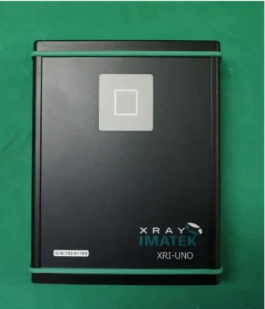
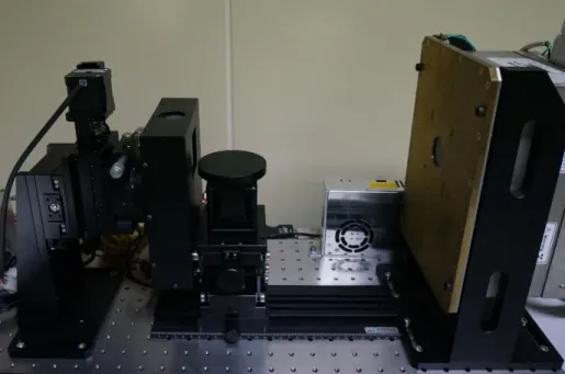
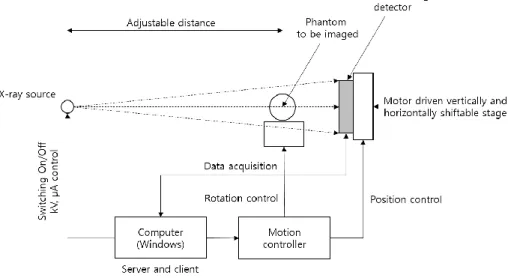
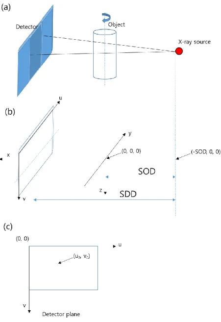
The developed CT system was composed of an X-ray source (SB-120- 350, Source-Ray Inc., Ronkonkoma, NY, USA), a photon-counting detector (Timepix, X-Ray Imatek, Barcelona, Spain) (Figure 3) (Table 1), and a rotational stage (Figure 4). The detector and the object stage could be moved vertically and horizontally with high precision by using a stepping motor (Ezi- STEP-PR-42M, Fastech Co., Bucheon, Korea). All of them are mounted on an optical bench in a shielded laboratory and controlled by a host computer. A schematic diagram of the system is shown in Figure 5. The source to detector distance (SDD) and source to object distance (SOD) are variable to change the magnification ratio, and field of view (FOV) of the system. In this system, the SDD was set to 285 mm, and the SOD was set to 235 mm with a geometric magnification ratio of 1.21. The detector was based on CMOS technology, has a 256 by 256 pixel matrix ASIC with a 55-μm pixel pitch. Every pixel of the ASIC had its own preamplifier, pulse shaper, 13-bit counter, and discriminator logic that included an adjustable threshold. The image data are transferred to the host computer by a USB serial cable.

The three-dimensional programmable stage consists of two motorized translation stages (SLS-80, Sciencetown, Incheon, Korea) and one motorized rotation stage (ST-AP11, Sciencetown, Incheon, Korea). The resolution of the

(24)

24

rotation stage is up to 0.0072 degree. The resolution of the translation stage is up to 0.02 μm. The FOV can be changed by shifting the position of the detector by using translation stage. The magnification ratio can be changed by adjusting the position of the object using optical rail stage, which will significantly affect the spatial resolution and the FOV.

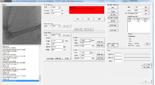
An integrated control software was developed. Automation of many of the used calibration techniques, such as alignment, noise floor calibration, and X-ray energy calibration, allows for a wider group of users to setup and operate the scanner (Figure 6).

(25)

25

Geometry Calibration

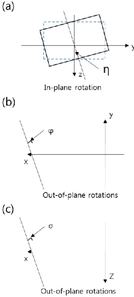
Precise geometric alignment is crucial to high quality imaging reconstruction in CT system. Several methods [43-45] have been proposed to evaluate and calibrate the geometric misalignment. In this scheme, rotation axis is defined as the Z axis of the system. The axis which pass through the X-ray focal spot and perpendicular to the Z axis is defined as the X axis. The axis perpendicular to the X-Z plane is defined as the Y axis (Figure 7). There are seven parameters to describe the system geometry:

(1) source to detector distance (SDD), (2) source to object distance (SOD),

(3) horizontal location of the intersection of the X axis and detector plane, u0,

(4) vertical location of the intersection of the X axis and detector plane, v0,

(5) in-plane rotation angle, the rotation angle of the detector plane along X axis, η

(6) out-of-plane rotation angle, the rotation angle of the detector plane along the axis of v=v0, σ

(7) out-of-plane rotation angle, the rotation angle of the detector plane along the axis of u=u0, φ

(26)

26

The two out-of-plane rotation angles, σ and φ, are quite difficult to determine with reasonable accuracy and have only a small influence on image quality, so σ and φ could be assumed to zero during geometric calibration, and then five other parameters need to be estimated (Figure 8).

Therefore, the method with multiple projection images acquired from rotating metal ball phantoms are used to estimate these five parameters[44].

(27)

27

Energy Calibration

The energy response of the detector was calibrated by using the X-ray tube’s potential as a reference. This technique was cross validated and practical for routine use in a research environment [46, 47]. The noise floor was measured. The noise floor of each pixel is caused by the overall noise contribution from sensor layer and readout electronics from preamplifier and shaper [48]. An integral noise floor scan was performed in the absence of radiation flux to establish the nose floor. The threshold scanning was performed over the range of 30–100 kVp in intervals of 10 kVp. For each of these energies, open-beam frames were obtained. A tube current of 10 μA and an exposure of 500 ms were used. A threshold corresponding to the selected kVp energy was selected where 50% of pixels are counting (on) Figure 15.

(28)

28

Figure 3. Photograph of the energy-resolved photon-counting X-ray detector.

(29)

29

Figure 4. Photograph of the developed multi-energy CT system consisting of a photon-counting detector, a movable rotational stage, and an X-ray tube.

(30)

30

Table 1. Specifications of the photon-counting detector.

Chip Size 1.61 × 1.41 cm²

Number of Pixels 256 × 256

Pixel Size 55 × 55 μm²

Sensor Area 14.1 × 14.1 mm²

Count Rate 1 MHz

Charge Collection e-, h+

Min. Detectable Charge ~2.7 KeV or ~750 e

Amplifier Gain ~18 mV / Ke

Noise ~75e

Threshold 1 (4 bits adj.)

Minimum Threshold ~500 e

Counter Depth / Overflow 14 bits / Yes Static Digital Power 200 mA @ 100 MHz

Readout Serial / Parallel

(31)

31

Figure 5. The functional schema of the experimental setup. It consists of a microfocus X-ray source, a photon counting detector and a shiftable stage. All of them are mounted on an optical bench and controlled by a host computer.

(32)

32

Figure 6. Screen shot of the developed integrated software GUI in action.

(33)

33

Figure 7. Geometry coordinate of proposed CT system.

(34)

34

Figure 8. Geometry parameters about rotation angle.

(35)

35

Data preprocessing, Image Reconstruction, and Postprocessing

The projection images were recorded in angle increments of 1.125 over 360 degrees for an acquisition time of 300 ms at 70 kVp and 300 μA per projection. By using photon-counting mode, I acquired multi-energy images by using energy thresholds of 32, 36, 40, 44, 48, 52, 56, and 60 keV. Thus, images from eight energy windows were available for material decomposition.

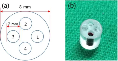
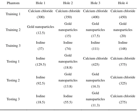
Cylindrical acrylic (PMMA) phantoms were fabricated 8-mm in diameter with four holes 2-mm each in diameter (Figure 9). In the training mode, the holes of the three phantoms were filled with the same materials, iodine, gold nanoparticles, and calcium chloride, at four different concentrations (Table 2).

In the test mode, the holes of an other three phantoms were filled with different materials at different concentrations (Table 2).

(36)

36

Figure 9. (a) A schematic drawing of the phantom 8-mm in diameter with four holes 2-mm in diameter containing four materials. (b) Photograph of the cylindrical PMMA phantom.

(37)

37

Table 2. Training and testing phantoms consisting of iodine, gold nanoparticles, and calcium chloride at different concentrations (mg/ml).

Phantom Hole 1 Hole 2 Hole 3 Hole 4

Training 1 Calcium chloride (300)

Calcium chloride (350)

Training 2 Gold nanoparticles (12.5)

Gold nanoparticles

(15)

Gold nanoparticles

(17.5)

Gold nanoparticles

(20) Training 3 Iodine

(37)

Iodine (74)

Iodine (111)

Iodine (148)

Testing 1 Iodine (129.5)

Gold nanoparticles

(18.8)

Gold nanoparticles

(13.8)

Gold nanoparticles

(16.3)

Iodine (55.5)

Gold nanoparticles

(11.3)

(38)

38

Analyzing the characteristics of photon counting detector and study of compensation method

As the detector pixels showed slightly different X-ray energy response functions, depending on the energy threshold and the projection frame sequence, I performed a different flat-field correction for each energy threshold and frame sequence. For each energy E and frame f, the flat-field correction was performed as follows:

f E f E f E

f E f E f

E

m

D F

D

C R

_,

, ,

,





 

(1)

,

CE f

: the corrected image for frame ^f, energy E, R: raw image, D: dark field image, F: flat field image, m^{E f}^,

: the average ofF^{E f}^, D^{E f}^, .

The ring artifact reduction method was also applied to the projection image [49]. The corrected projection image was converted into a log- normalized projection, which was reconstructed by using the FDK algorithm [50].

For a further reduction of the noise, the reconstructed image was processed by using bilateral filtration, which is an effective edge-preserving smoothing filter that factors in the Euclidean distance and radiometric differences in neighboring voxels [51]. A bilateral filter was used to suppress the noise of the micro CT images for material decomposition [15, 52].

(39)

39

Material Decomposition Using the Attenuation Coefficient Ratio and MDA

In spectral CT imaging, the measured linear attenuation coefficient

( , )

L

E x

n



at spatial coordinate x in the energy bin En depends on the

concentration



_i

( ) x

and the mass attenuation coefficient



_{M i}_,(E_n) of the constituent material i as follows:

Let us assume that the partial volume effect is negligible, each voxel can be treated as consisting of a single material. In this case,



_L

( E x

_n

, )

depends on the attenuation of a single material. As such, the attenuation coefficient ratio



_R

( E

_n

)

is independent of material concentration at each energy bin.





 ^K

i

n i M i n

L E x x E

1

,( )

) ( )

,

(

 



^ ^ (2)

) (

) ) (

(

1



n L

n L n

R E

E E



  (3)

The vector

x

is composed of attenuation coefficient ratios and is measured at multi-energy bins for voxels.

)) ( ..., ), ( ), (

(

₁ ₂ _₁

 

_R

E 

_R

E 

_R

E

_n

x

⁽⁴⁾

(40)

40

The material decomposition algorithm was divided into an identification task and a quantification task. Material decomposition strategy is shown in Figure 10. I first identified the material by using the vector of attenuation coefficient ratios and subsequently determined its concentration.

The material’s multi-dimensional attenuation ratio vector was used as a feature vector for identification. I used the MDA algorithm to classify the feature vectors of the materials. Let

x

ⁱ_j be a seven-dimensional column vector that denotes the j-th sample from the i- th material; then

} ,..., , ,..., ,

{

¹₁ ¹₂ ¹ ₁²

1

C N

N _C

X  x x x x x

contains all the training samples. The vector of the optimal projection matrix, W, can be represented by using a linear transformation as

x W

y 

^T . (5)

In the intra-class covariance matrix for the number of classes, c, is calculated from

S

,

1





 ^c

i i

W S (6)

x x x x

x

, ) )(



(



 

i

i i

i - -

S

 (7)

1



,



 N i

i

 x

x

₍₈₎

(41)

41 and the inter-class covariance matrix by using

x x x x

S

( )( ) ,

1





 



 ^c

i

i i

i

B N (9)

1 .

1

 







i

i i c

N N

N _x

x

_x _

x

₍₁₀₎

In order to separate the classes, I find a projection matrix (W^*) that maximizes

W S W

W S W W

W T

B T

J( ) . (11)

The optimal projection matrix maximizes the inter-class variation and minimizes the intra-class variation. The projection matrix must be initially calculated from known material samples. Finally, the identification of a new material is performed by minimizing the Euclidian distance between material vectors, after projection via the optimal projection matrix.

For quantification of the concentration, a relationship between attenuations (μL) at multiple energy bins and concentrations (ρm) was fitted linearly by using the unweighted least-squares method for each material:

(42)

42







 ^N

n

n m n L n m

m a E b

N1 ₁ ^, ( ) ^,





^. (12)

The fitted model was used to calculate the concentrations from the linear attenuations of the identified material.

(43)

43

Evaluation of Material Decomposition Performance

The performance of material identification was evaluated in terms of true positive (TP), true negative (TN), false positive (FP) and false negative (FN). The corresponding circular ROIin and annular ROIout with the same areas were defined for each hole in the slice images (Figure 27). The two ROIs were separated by a narrow annular region with thickness equal to 4% of the hole’s diameter in order to avoid partial volume effects [53]. The voxels correctly identified as the true material were measured as TP, and the voxels incorrectly identified as the true material were measured as FN in the ROIin. The voxels correctly identified as PMMA were measured as TN, and the voxels incorrectly identified as PMMA were measured as FP in the ROIout. The performance of material identification was calculated as sensitivity (Sens), specificity (Spec) and accuracy (Acc):

2 Spec Acc Sens

FP, TN Spec TN FN, TP

Sens TP 

 

 (13)

The quantification performance was evaluated as a percentage error of the measured concentration compared with the true value.

(44)

44

Figure 10. Flowchart of the material decomposition and quantification strategy.

(45)

45

RESULTS

Multi-energy CT System

The fractions of on pixels were calculated in energy ranges from 30 to 100 kVp (Figure 15). The energy calibration by using the X-ray kVp and the threshold technique provided good agreement, which yield R² = 0.9971 (Figure 16). I imaged the cylindrical phantom of PMMA with four holes filled with iodine, gold nanoparticles, and calcium chloride. Without any filtering the reconstructed image of the phantom displays ring artifacts in the central region and other artifacts in the peripheral region (Figure 21(a), (f), (k)). The ring artifacts were more conspicuous in the reconstructed images by using some energy thresholds, then they were in other; which was caused by the different energy response functions of the pixels. In the reconstructed images after the flat field correction by using a single projection frame, the ring artifact was reduced, though much remained (Figure 21(b), (g), (l)). By using our flat-field correction method, I was able to reduce the ring artifacts considerably (Figure 21(c), (h), (m)). The noise was further reduced after ring artifact reduction (Figure 21(d), (i), (n)) and bilateral image filtering (Figure 21(e), (j), (o)). Figure 22 shows the final reconstructed images for different energy thresholds after all filter processing; these were used for material decomposition.

(46)

46

Figure 11. (a) Geometry calibration phantom consists of eleven ball bearings with 1-mm diameter. (b) Projection image of ball bearing phantom at the leftmost position. (c) Projection image of ball bearing phantom at the rightmost position. (d) The position values of trajectory tracking.

(47)

47

Figure 12. (a) Projection image of ball bearing phantom at the farthest position from the X-ray source. (b) Projection image of ball bearing phantom at the nearest position from the X-ray source. (c) Position differences in pixel between the farthest position and the nearest position was calculated.

(48)

48

Figure 13. X-ray tube spectrum measured using photon counting detector for various kVps. The tube current of 10 μA and exposure time of 500 ms were used.

300 400 500 600 700 800 900 1000

0 1 2 3 4 5 6x 10⁷

Threshold

Number of photons

30 kVp 40 kVp 50 kVp 60 kVp 70 kVp 80 kVp 90 kVp 100 kVp

(49)

49 Figure 14. The noise floor threshold scan.

1500 200 250 300 350 400

1 2 3 4 5 6 7x 10⁴

Threshold

Number of Pixels Counting > 10

(50)

50

Figure 15. Threshold scan for varying X-ray source energies from 30 to 100 kVp. Thresholds where 50% pixels are on were selected as energy calibration points.

(51)

51

Figure 16. Threshold-energy calibration performance using the X-ray kVp reference

method.

(52)

52

Figure 17. Flat field corrected images. (a) Raw flat field image. (b) Dead or hot pixel corrected image. (c) Flat field corrected image. Sample phantom image (d) without flat field correction, (e) with dead or hot pixel correction, and (f) with flat field correction.

(53)

53

Figure 18. Flat field corrected images of material phantom by using multiple frames. Processing methods: (a) without flat field correction, (b) flat field correction using single frame, (c) flat field correction using multiple frames.

(54)

54

Figure 19. Ring artifact correction was performed in sinogram domain.

Sinogram consists of all 320 measured projection data. (a) Sinogram exposes line artifacts that are responsible for ring artifacts. (b) Sinogram after removing line artifacts. (c) Reconstructed image of test phantom from the sonogram (a).

In this image ring artifacts are clearly visible. (d) After ring artifacts correction.

The image is reconstructed from the sonogram (b).

(55)

55

Figure 20. (a) Raw image, and denoised images by using bilateral filtration by sigma value of (b) 0.5, (c) 2, and (d) 3, respectively. Window size of (1) 3×3, (2) 4×4, and (3) 5×5 were used.

(56)

56

Figure 21. Reconstructed multi-energy images of a testing phantom, (a, f, k) with no flat field correction, (b, g, l) with a conventional flat field correction, (c, h, m) with a flat field correction using multi-frames, (d, i, n) with ring artifact reduction filtering, and (e, j, o) with bilateral filtering at (a-e) 32-keV, (f-j) 48-keV, and (k-o) 60-keV energy thresholds.

(57)

57

Figure 22. Multi-energy images of a testing phantom used for material decomposition at (a) 32-keV, (b) 36-keV, (c) 40-keV, (d) 44-keV, (e) 48-keV, (f) 52-

keV, (g) 56-keV, and (h) 60-keV energy thresholds. Hole 1 was filled with iodine (129.5 mg/ml), hole 2 with gold nanoparticles (18.8 mg/ml), hole 3 with calcium chloride (425 mg/ml), and hole 4 with calcium chloride (375 mg/ml).

(58)

58

Table 3. Time taken by single-core CPU implementation to reconstruct volumes of

varying dimensions from 320 projection images.

Volume File I/O Filter Time Backprojection

Time Total Time

128³ 2.94 s 2.64 s 42.36 s 47.94 s

256³ 9.97 s 7.92 s 169.40 s 187.19 s

512³ 54.72 s 24.52 s 673.80 s 753.04 s

(59)

59

Table 4. Time taken by multi-core CPU implementation to reconstruct volumes of varying dimensions from 320 projection images.

Time Total Time

128³ 0.29 s 0.87 s 8.42 s 9.58 s

256³ 0.33 s 2.03 s 33.69 s 36.05 s

512³ 0.38 s 6.13 s 174.88 s 181.39 s

(60)

60

Table 5. Time taken by GPU implementation to reconstruct volumes of varying dimensions from 320 projection images.

Time Total Time

128³ 2.47 s 1.04 s 4.76 s 8.27 s

256³ 5.07 s 2.02 s 34.11 s 41.20 s

512³ 10.33 s 6.16 s 163.07 s 179.56 s

(61)

61

Multiple Discriminant Analysis of material phantom

For training and testing using MDA decomposition, I imaged the six cylindrical phantoms described in Table 2. The holes in three cylinders were filled with the same material at different concentrations for MDA training, and those in another three cylinders were filled with different materials at different concentrations for MDA testing. For the training phantom, the effective linear attenuation values were measured at pixels in an ROI, and average values over pixels were calculated for each material and each energy threshold. Figures show the attenuation coefficient curves for iodine (Figure 23), gold nanoparticles (Figure 24), and calcium chloride (Figure 25) according to the energy threshold. The curves of effective linear attenuations were proportional to the material’s concentration. The linear attenuation curve of iodine does not demonstrate a strong discontinuity around the K-edge (33.2 keV) (Figure 23).

Calcium-chloride attenuation demonstrates a strong decrease with increasing energy (Figure 25). This behavior is typical of medium-Z materials, where the attenuation is dominated by photoelectric effects at lower energies. Therefore, this material is more visible in lower energy ranges. The attenuation of the light material PMMA is dominated by Compton scattering, and the dependence on energy is much weaker (Figure 25). The figure shows only a slight difference in the effective linear attenuation coefficient according to energy bins. Figure 26 shows attenuation coefficient ratios at multi-energy bins. The same material shows similar linear attenuation coefficient ratio curves regardless of its concentration, and different materials show patterns different from one another.

(62)

62

The ratio value of the linear attenuation demonstrates a much larger difference between materials when the energy exceeds 48 keV.

For the testing phantoms (Table 2), the multi-dimensional ratio vector of the materials at all voxels was classified into four materials by using a MDA.

The result for material identification by applying the MDA to a testing phantom is shown in Figure 27. This method produces binary images for each material based on the assumption that each voxel contains predominantly one material.

Some regions of mis-identification are present at edges of holes due to a partial volume effect. The overall performance of material decomposition by using the MDA in the testing phantoms is shown in Table 6.

The mean accuracies for the three phantoms were 0.88±0.05, 0.96±0.06, and 0.99±0.01. The mean accuracies for the materials were 0.94±0.03 for iodine, 0.96±0.02 for gold nanoparticles, and 0.92±0.05 for calcium chloride. For voxels in the material-specific ROI after identification, the concentrations were determined by using the least-squares method (Table 7). The measured concentration of the voxels was quantified by using a pseudo- color coding of the corresponding value (Figure 28). The mean percentage errors were 1.90±1.58% for iodine, 3.85±3.13% for gold nanoparticles, and 3.40±2.62% for calcium chloride over different concentrations in the three phantoms.

(63)

63

Figure 23. Measured energy-dependent attenuation coefficients of (a) iodine, (b) gold nanoparticles, and (c) calcium chloride at four different concentrations in the testing phantoms.

(64)

64

(65)

65

(66)

66

Figure 26. Means and standard deviations of the attenuation coefficient ratios for gold nanoparticles, iodine, calcium chloride, and PMMA from the testing phantoms.

(67)

67

Figure 27. Decomposed images for (a) gold nanoparticles, (b) calcium chloride, (c) iodine, and (d) PMMA in a testing phantom. ROIs of the same areas are selected inside (ROIin) and outside (ROIout) of each hole for calculating the sensitivity, specificity, and accuracy.

(68)

68

Figure 28. Concentration quantification of (a) testing phantom 1, (b) testing phantom 2, and (c) testing phantom 3 with gold nanoparticles shown in red, calcium chloride in green, and iodine in blue by using pseudo-color coding.

(69)

69

Table 6. Overall performance of material decomposition in the three testing phantoms.

Phantom Material Concentrations

(mg/ml) Sensitivity Specificity Accuracy

Testing 1

Iodine 129.5 0.79 0.84 0.82

Gold

nanoparticles 18.8 0.88 0.83 0.85

Calcium chloride 425 0.98 0.85 0.92

Testing 2

Iodine 92.5 1.00 1.00 1.00

Gold

nanoparticles 13.8 0.99 0.99 0.99

Gold

nanoparticles 16.3 0.99 0.99 0.99

Testing 3

Iodine 18.5 0.97 1.00 0.98

Iodine 55.5 0.95 1.00 0.98

Gold

nanoparticles 11.3 0.99 0.98 0.99

(70)

70

Table 7. Results of concentration quantification of the materials from the three testing phantoms.

Material Nominal (mg/ml) Measured (mg/ml) Percentage error (%)

Iodine

129.5 128.53±0.43 0.75

92.5 91.67±0.52 0.90

55.5 54.52±0.60 1.77

18.5 17.73±0.74 4.16

Gold nanoparticles

18.8 18.86±0.18 0.59

16.3 13.51±0.16 6.58

13.8 17.32±0.21 1.75

11.3 10.52±0.35 6.49

Calcium chloride

425 450.68±0.94 6.04

375 370.78±4.30 1.13

325 328.78±5.81 1.16

275 289.49±6.39 5.27

(71)

71

DISCUSSION

Two types of approaches are need to decompose specific materials by using multi-energy CT images: one is to decompose in the projection image domain [6, 26], and the other in the reconstructed image domain [27, 28].

Although decomposition in the projection domain is beneficial for removing the beam hardening effect, this method requires careful calibration of the attenuation functions and energy response of the imaging system. The K-edge [30], least-squares parameter estimate [31], and singular value decomposition (SVD) methods [32] have been used to decompose basis materials in the projection image domain [31, 33, 34]. However, these methods have some limitations. The K-edge method cannot be used to discriminate between materials that do not have a K-edge in the energy range of interest, and the least- squares estimate and the SVD methods are vulnerable to noise. A tunable monochromatic X-ray source or simulation tools are required to obtain an energy response function. However, a tunable monochromatic X-ray source requires large and expensive facilities, such as a synchrotron, and are hence not appropriate for routine use. Further, relying on the use of simulation data is not desirable as this can cause estimate errors, and may fail to consider the aging effect of the detector [35]. As an alternative to the decomposition method in the projection image domain, one can use reconstructed images from each of the energy windows to decompose the object into various materials or regions. An advantage of material discrimination in reconstructed images is that it is quick and straightforward. In our approach, identification by using the MDA and concentration quantification was performed under the assumption that each

(72)

72

voxel consisted primarily of one material. Therefore, higher-quality volume images can improve discrimination accuracy; these can be obtained from lower- dose projection images by using advanced iterative reconstruction techniques, instead of the FDK technique used.

Existing energy calibration techniques employ monochromatic photon sources such as radio-isotopes [54-57], synchrotron [58, 59], and X-ray flurorescence (XRF) from metallic targets^[59-61]. Each of these methods has limitations that reduce their usefulness in pre-clinical or clinical applications such as special setup of equipment, long measurement time, and physical space required for maintaining the proper geometry of X-ray, detector, and target metallic foils. Also, radio-isotopes are not readily available in a small laboratory and frequent use of them may not be justifiable from the radiation protection point of view. To overcome the limitations of existing energy calibration techniques, this study calibrated by using the X-ray tube’s potential.

Previous studies have used statistical information obtained from spectral CT images to show energy-dependent variations in materials via PCA [36, 37]. Both PCA and MDA are linear projection processes and are closely related. The PCA is a linear transformation that identifies the axis that enlarges dataset deviation. In contrast to the PCA, which ignores class information, the MDA is a linear transformation that identifies the axis that widens the partition between different classes. That is, the PCA finds the axes with maximal deviations, where the data are most distributed, and the MDA additionally maximizes the spread between classes. Therefore, the MDA can be used to yield a lower-dimensional signal amenable to material classification [39]. To

(73)

73

date, study of material identification for spectral CT images has been conducted using the MDA method. In this study, for training, the material attenuation coefficient ratio was calculated by using an application-specific phantom. As the optimal material discrimination matrix is application specific in the MDA, the optimization approach may not be robust to noise. Although scattering noise in the object or detector is not a major concern in imaging small-size objects [62], the noise depends on the specific phantom’s configuration in a reconstructed image. That is, the discrimination (covariance) matrix was applied to image classes of known context in this study. As a consequence, the MDA partitioned the feature space into class-labeled decision regions with high accuracy. In this study, the ROIs composed entirely of a single material were arbitrarily selected in several slices by an operator. Therefore, the ROIs selected for training had different noise levels that influenced the discrimination matrix and accuracy.

In previous studies, the identification of multiple materials was studied based on different approaches by using photon-counting spectral CT.

The typical method begins by designing a system of equations considering multi-energy data sets and uses attenuation coefficient functions for decomposition. Iteratively solving the system of equations results in the identification of materials with K-edges inside the radiological energy range [30, 33]. Although this approach can efficiently discriminate between materials, the design of a reliable and robust system of equations that avoids the ill-posed problem and the divergence problem is essential. As this method is highly sensitive to errors in the forward model in the projection space, they require

(74)

74

accurate calibration and high stability in the detector response function over time. When solving the system of equations, iterative calculations for each element in the projection image are also required. A large number of repetitive calculations must be performed to estimate the final contributions of the materials for each pixel. Consequently, whether material decomposition using iterative methods suits clinical applicability, in context of the required processing time, must be carefully considered. Contrary to iterative methods, our approach can identify multiple materials based on an optimal projection matrix calculated without iteration. Moreover, in contrast to methods directly using attenuation coefficient decomposition, our method does not require prior knowledge of either the constant on the coefficients of particular functions, including the photoelectric, Compton, and detector response functions.

Photon-counting detectors have several limitations, such as charge- sharing and pulse pile-up effects. Although charge-sharing between neighboring pixels can cause degradation of image quality and loss of spectral information [63], the detector used in this study has already been validated as a relevant tool for the energy-sensitive radiography of soft materials [63-65]. In our experiment, the attenuation curves did not appear to be ideal curves for several reasons: energy bin width, charge sharing, spectral response of the CdTe detector, source spectrum, and inevitable noise. These all combined to make the measured attenuation plots non-ideal, and no resultant sharp attenuation jump, as in the iodine K-edge, was observed. Despite these unfavorable conditions, the feature vectors of the attenuation coefficient ratios showed sufficient ability to discriminate materials in different classes.

(75)

75

The objective of this study was to develop both a spectral CT system by using a photon-counting detector and a new method to identify materials by using attenuation coefficient ratios. The material-specific ratios did not depend on the concentrations of materials, but on the mass attenuation coefficients according to energies. The MDA method identified materials in the reconstructed image domain, and the concentrations of the four materials were quantified by using the least-squares method. Iodine, gold nanoparticles, calcium chloride, and PMMA were separated and quantified accurately. I will apply the developed spectral CT system and decomposition method to material decomposition of in-vivo multi-energy animal images in future studies.

(76)

76

REFERENCES

[1] L. Yu, X. Liu, S. Leng, J. M. Kofler, J. C. Ramirez-Giraldo, M. Qu, et al., "Radiation dose reduction in computed tomography:

techniques and future perspective," Imaging in medicine, vol. 1, pp. 65-84, 2009.

[2] X. Wang, D. Meier, K. Taguchi, D. J. Wagenaar, B. E. Patt, and E.

C. Frey, "Material separation in x-ray CT with energy resolved photon-counting detectors," Med Phys, vol. 38, pp. 1534-46, Mar 2011.

[3] T. J. Vrtiska, N. Takahashi, J. G. Fletcher, R. P. Hartman, L. Yu, and A. Kawashima, "Genitourinary Applications of Dual-Energy CT," AJR. American journal of roentgenology, vol. 194, pp. 1434- 1442, 2010.

[4] T. Xu, J. L. Ducote, J. T. Wong, and S. Molloi, "Feasibility of real time dual-energy imaging based on a flat panel detector for coronary artery calcium quantification," Med Phys, vol. 33, pp.

1612-22, Jun 2006.

[5] J. G. Fletcher, N. Takahashi, R. Hartman, L. Guimaraes, J. E.

Huprich, D. M. Hough, et al., "Dual-energy and dual-source CT:

is there a role in the abdomen and pelvis?," Radiol Clin North Am, vol. 47, pp. 41-57, Jan 2009.

(77)

77

[6] R. E. Alvarez and A. Macovski, "Energy-Selective Reconstructions in X-Ray Computerized Tomography," Physics in Medicine and Biology, vol. 21, pp. 733-744, 1976.

[7] X. W. Wang, J. M. Li, K. J. Kang, C. X. Tang, L. Mang, Z. Q. Chen, et al., "Material discrimination by high-energy x-ray dual- energy imaging," High Energy Physics and Nuclear Physics- Chinese Edition, vol. 31, pp. 1076-1081, Nov 2007.

[8] K. V. Haderslev and M. Staun, "Comparison of dual-energy x- ray absorptiometry to four other methods to determine body composition in underweight patients with chronic gastrointestinal disease," Metabolism-Clinical and Experimental, vol. 49, pp.

360-366, Mar 2000.

[9] M. Petersilka, H. Bruder, B. Krauss, K. Stierstorfer, and T. G.

Flohr, "Technical principles of dual source CT," European Journal of Radiology, vol. 68, pp. 362-368, Dec 2008.

[10] Y. Zou and M. D. Silver, "Analysis of fast kV-switching in dual energy CT using a pre-reconstruction decomposition technique,"

in Medical Imaging, 2008, pp. 691313-691313-12.

[11] X. Llopart, M. Campbell, R. Dinapoli, D. S. Segundo, and E.

Pemigotti, "Medipix2: a 64-k pixel readout chip with 55 mu m square elements working in single photon counting mode," Ieee Transactions on Nuclear Science, vol. 49, pp. 2279-2283, Oct 2002.

(78)

78

[12] K. Taguchi and J. S. Iwanczyk, "Vision 20/20: Single photon counting x-ray detectors in medical imaging," Med Phys, vol. 40, p. 100901, Oct 2013.

[13] S. D. Sordo, L. Abbene, E. Caroli, A. M. Mancini, A. Zappettini, and P. Ubertini, "Progress in the Development of CdTe and CdZnTe Semiconductor Radiation Detectors for Astrophysical and Medical Applications," Sensors (Basel), vol. 9, pp. 3491-526, 2009.

[14] D. P. Cormode, P. E. Roessl, P. A. Thran, P. T. Skajaa, B. R. E.

Gordon, P. J.-P. Schlomka, et al., "Atherosclerotic Plaque Composition: Analysis with Multicolor CT and Targeted Gold Nanoparticles," pp. 1-9, Jul 29 2010.

[15] J. R. Ashton, D. P. Clark, E. J. Moding, K. Ghaghada, D. G. Kirsch, J. L. West, et al., "Dual-energy micro-CT functional imaging of primary lung cancer in mice using gold and iodine nanoparticle contrast agents: a validation study," PLoS One, vol. 9, p. e88129, 2014.

[16] T. G. Schmidt, "CT energy weighting in the presence of scatter and limited energy resolution," Medical Physics, vol. 37, p. 1056,