Effects of Growth Controls on Homebuilding in California Local Jurisdictions : Focusing on the late 1980s

(1)

1. Introduction

In the past three decades, the United States has witnessed the spread of growth management and control measures (henceforth, growth controls).¹⁾A large number of localities, especially in suburbs, has

enacted the measures to tackle economic and environmental problems (e.g., increasing tax burden and loss of open space) induced by rapid suburban growth (Dowall 1979). In the process, such locally enacted growth controls have potentially influenced U.S. suburbanization by regulating housing construc-

* Ph.D. Candidate, Department of Geography and Regional Development, University of Arizona, Tucson, AZ 85721, U.S.A., pillsung@email.arizona.edu

Effects of Growth Controls on Homebuilding in California Local Jurisdictions: Focusing on the late 1980s

Pillsung Byun*

캘리포니아 주내 지방정부의 성장관리 규제가 주택건설에 미치는 영향에 관한 연구: 1980년대말을 중심으로

변 필 성*

Abstract : This paper discusses the price effects of local growth controls on the housing markets of California jurisdictions in the late 1980s empirically. Particularly, based on spatial econometric modeling, the study focuses on the homebuilding constrained by growth controls which is one of the price effects. The modeling produces the California-wide generalizable results, differentiates among the individual effects of various growth controls on homebuilding, and covers spatial effects. Thereby, this study intends to supplement the existing works on the price effects of growth controls. The modeling results find that restrictive residential zoning had the effect of significantly restricting housing construction in the late 1980s. On the other hand, urban growth boundaries had the effect of accommodating homebuilding. Population growth or housing permit caps and adequate public facility ordinances had no significant effects on housing construction.

Key Words : growth controls, price effects, homebuilding, California, spatial econometric modeling

요약: 본 연구는, 미국 지방정부의 성장관리 규제가 유발시키는 지역주택시장내 가격상승효과를 이해하기 위해,

성장관리가 가질 수 있는 주택건설 억제 효과를 실증적으로 분석했다. 실증 분석은1980년대말 캘리포니아내 지방 정부를 대상으로 했으며, 공간계량경제 모델을 활용했다. 분석을 통해, 본 연구는 성장관리의 주택가격상승효과에 관한 기존 연구의 한계를 극복하는 데 기여하고자 했다. 즉, 캘리포니아 주와 같은 비교적 광범위한 지역에 적용 되는 일반화된 결과를 얻었고, 개별 성장관리 규제가 주택건설에 미치는 영향력을 고찰했으며, 아울러 공간효과, 특히 공간적 자기상관을 분석모델에 반영시킴으로써 분석의 설명력을 제고했다. 모델링 결과, 주거용도지역내 허 용개발밀도를 저하시키려는 일련의 성장관리규제는 주택건설을 억제시키는 효과를 보였다. 하지만, 주택건설 및 도시성장을 지방정부가 설정한 지역내에 한정시키는 규제는, 오히려, 주택건설을 증가시키는 효과를 보였다. 연간 인구증가 및 건축허가건수를 제한하는 규제와 주택건설업자의 공공하부구조 공급을 강제하는 법규는 주택건설에 유의한 영향을 미치지 않은 것으로 나타났다.

주요어 : 성장관리, 가격상승효과, 주택건설, 캘리포니아, 공간계량경제 모델링

(2)

tion and residential (re)location in suburbs.

Specifically, by raising housing construction costs and inflating housing prices, local growth controls affect housing markets of the jurisdictions implementing the control measures (Dowall 1984) - the price effects of growth controls. As a result, prospec- tive residents and homebuilders are priced out and forced out of the jurisdictions, respectively. Such residents and homebuilders have to shift to neighboring jurisdictions with no, or less stringent, growth controls - spillovers occurs (Dowall 1984). Amid the diffusion of growth controls since the 1970s, spillovers have likely progressed across metropolitan regions of U.S., and thereby contributed to suburbanization (Carruthers and Ulfarsson 2002; Byun and Esparza 2003). Significantly, the likely contribution of spillovers to suburbanization is based on the effects of local growth controls on housing markets, the price effects. For this reason, an investigation of the impacts of growth controls on local housing markets can be an important basis for studies of the potential impacts of growth controls on U.S. suburbanization.

Since the 1970s, not a few empirical works have dealt with the effects of growth controls on local housing markets (Janczyk and Constance 1980; Elliot 1981; Schwartz et al. 1981; Schwartz et al. 1984;

Landis 1986; Katz and Rosen 1987; Pollakowski and Wachter 1990; Singell and Lillydahl 1990; Thorson 1997; Skidmore and Peddle 1998; Levine 1999;

Mayer and Somerville 2000; Pendall 2000).

However, these previous studies have showed limitations - few region-wide generalizable results, little differentiation among individual effects of various growth controls, use of inadequate spatial units, little consideration of spatial effects in empirical modeling, and use of an insufficient indicator.

This study attempts to overcome such limitations for effectively analyzing the effects of growth controls on housing markets. Specifically, my study seeks to differentiate among the individual effects that various growth controls have on local housing construction. In order to cover the possible spatial

effects (spatial autocorrelation) with respect to local homebuilding, my work employs spatial econometric modeling. The modeling targets the local jurisdictions of California in the late 1980s.

Following this introduction, the second chapter discusses growth controls, the price effects of growth controls, and the limitations of the existing studies.

The limitations re-emphasize and specify the research objectives of this paper. Such re-emphasis and specification in turn guides an empirical analysis, the third chapter. The empirical portion presents study area, data, models, and the discussion of modeling results. The fourth chapter concludes this paper by summarizing the results and suggesting future research subjects.

2. Growth Controls and Price Effects

The first two sections of this chapter describe the four types of local growth controls that this study deals with, and then discuss how the controls raise housing and prices and construction costs. The third section reviews the existing empirical studies of the price effects.

1) Growth Controls

The growth controls that my study uses include population growth or housing permit caps, urban growth boundaries, adequate public facility ordinances (henceforth APFOs), and restrictive residential zoning. These controls are applied to housing construction.

First, population growth or housing permit caps limit the amount of population inflow or housing construction by applying an annual quota to building permit issuance (Landis 1992; Pendall 2000). The difference between population growth and housing permit caps depends on whether or not the annual quota of housing permits is fixed. While housing permit cap fixes the quota for a predetermined period, population growth cap limits the amount of housing permits in accordance with an annual target

(3)

of population inflow. Local jurisdictions enact these caps to slow unanticipated population growth.

Second, urban growth boundaries contain growth (or housing construction) within designated areas by not providing public infrastructure to the residential development outside the boundaries for predetermined periods (Nelson and Moore 1993; Pendall 2000). This control is basically used to attack sprawl - to preserve prime farmland or resource land and to promote in-fill and high-density development (Dawkins and Nelson 2002).

Third, adequate public facility ordinances (APFOs) force homebuilders or developers to supply sufficient public infrastructure to minimize the impacts of their new development on existing infrastructure (Levy 2000). In reality, APFOs make development approval contingent upon a local government’s evaluation of public infrastructure supplied by homebuilders or developers (Pendall 2000).

Fourth, restrictive residential zoning seeks to sup- press permitted residential density on given residen- tially zoned land (Pendall 2000). Specifically, this control includes large minimum-lot requirement and rezoning of residential land to less intense uses such as open space or agriculture. Furthermore, the control can encompass the measures to require voter approval or local legislature’s super-majority approval for the amendments of zoning ordinances or general plans that allow residential density increases. This delimitation of restrictive residential zoning is based on the classification of growth controls used in the 1988 survey of local growth controls in California (for the survey results, see Glickfeld and Levine 1992).

2) Price Effects of Growth Controls Local growth controls lead to housing price inflation in localities. Specifically, the housing price inflation is generated through rising construction costs, restricted supply of new housing, improved amenities, and market reorientation towards upscale housing. These four ways how growth controls raise

housing prices constitute the price effects of growth controls. At the general level, the price effects are discussed below.

First, growth controls increase housing construction costs, and the rising costs inflate prices of new housing (Dowall 1979; Elliot 1981; Schwartz et al.

1981; Dowall 1984; Landis 1986; Zorn et al. 1986; Katz and Rosen 1987; Lillydahl and Singell 1987; Singell and Lillydahl 1990; Levine 1999; Mayer and Somerville 2000; Luger and Temkin 2000).

Specifically, local growth controls raise construction costs in the following ways:

• By delaying regulatory procedures, growth controls increase financial costs, and heighten uncer- tainty concerning the outcome or length of regulatory processes.²⁾Additionally, since such delayed procedures prevent homebuilders from flexibly adjusting to changes in market condition, homebuilders can face opportunity costs from “missing the market”(Luger and Temkin 2000, 4).

• Local growth controls constrain land supply, and increase land costs. For example, urban growth boundaries can have the effects of constraining land supply by containing housing construction within the boundaries (Nelson 1985). And, in the case of downzoning of residential land to less intense uses, supply of residential land for homebuilding will likely be constricted.

• Local growth controls generate inefficiency in homebuilding operations. For instance, large minimum-lot requirement reduces maximum possible amount of housing construction on given land.

Housing permit cap issues less amount of building permits than homebuilders demand. In these cases, given fixed costs like land costs, homebuilders cannot pursue economies of scale, and construction cost per housing unit will likely increase.

• The required provision of infrastructure and facilities as exactions can increase construction costs.

This is pertinent for APFOs.

Second, local growth controls constrain supply of new housing (Dowall 1984; Landis 1986; Lillydahl

(4)

and Singell 1987; Singell and Lillydahl 1990;

Skidmore and Peddle 1998; Levine 1999; Nelson et al.

2002). Rising construction costs and reduction of profitability by local growth controls force incum- bent homebuilders out of markets (Rosen and Katz 1981). Moreover, many homebuilders move to other localities without growth controls in order to reduce costs (Levine 1999). As a result, supply of new housing is constrained, and housing price inflation unfolds. Furthermore, such inflation is not easily mitigated because local growth controls prevent homebuilders from adjusting housing construction to the rise in housing prices (Frieden 1979; 1983).

This is revealed by the low elasticity of new housing construction to price increase (Mayer and Somerville 2000) that appears in growth-controlled localities.

Third, local growth controls enhance neighborhood amenities, and thereby increase housing prices (Dowall 1984; Schwartz et al. 1981; Landis 1986;

Lillydahl and Singell 1987; Singell and Lillydahl 1990; Skidmore and Peddle 1998; Levine 1999; Luger and Temkin 2000; Nelson et al. 2002). Since growth controls are used to minimize urban growth- induced costs (e.g., traffic congestion, noise, crime, and loss of open space), amenities are improved, and housing prices are increased because amenities belong to the features of housing influencing housing prices. Moreover, such enhanced neighborhood amenities stimulate additional housing demand from the middle-or-upper-class (Schwartz et al.

1981), thereby fueling housing price increase.

Fourth, housing construction costs increased by growth controls make homebuilders switch their target markets to the high-priced housing for high- income homebuyers (Dowall 1979; Dowall 1984;

Schwartz et al. 1984; Landis 1986; Nelson et al. 2002;

Pendall 2000). Such market reorientation serves as a business strategy offsetting the rise in cost per housing unit and the resulting reduction of profitability.

In this situation, housing price inflation is reinforced.

Housing affordability becomes a problem because the market reorientation creates significant barriers to

even moderate-income homebuyers (Dowall 1984).

3) Existing Studies of the Price Effects of Growth Controls

Many empirical studies of the price effects of growth controls have come out while growth controls spread across many metropolitan regions of U.S. since the 1970s. This section describes characteristics of the existing studies, focusing on their limitations.

First, many existing works focus on one growth control enacted in a single locality or several jurisdictions, especially using time-series data of housing prices or supply (see Janczyk and Constance 1980;

Schwartz et al. 1984; Singell and Lillydahl 1990;

Thorson 1997; Skidmore and Peddle 1998). These works are of much value as case studies. However, they are of limited value in producing region-wide (e.g., statewide) generalizable results.

Second, even so, the existing studies enabling region-wide generalization have the following limitations:

• The individual price effects of various growth controls are not differentiated (see Elliot 1981; Katz and Rosen 1987). For this reason, such studies cannot empirically discuss how much each growth control inflate housing prices or constrain homebuilding and whether or not each control takes a significant effect, compared to other controls.

• By using spatial units (e.g., Metropolitan Statistical Areas and counties) that are larger than political entities - local jurisdictions - implementing growth controls, many studies fail to accurately capture the price effects (see Mayer and Somerville 2000).

If such spatial units are used, potential processes within the spatial units - the price effects of one jurisdiction’s growth controls and the resulting spillovers towards neighboring jurisdictions - are overlooked.

• Spatial effects or spatial dependencies are not cov- ered, although spatial data are used for many analyses (see Levine 1999; Pendall 2000). Spatial effects can occur through the interaction among

(5)

adjoining jurisdictions or the mismatch between data aggregation units and realistic spatial scope of data generating processes (see Anselin 1988, Florax et al. 2002, and Florax and Nijkamp 2004, for spatial effects or dependence in modeling). In relation to modeling, such spatial effects are embodied in spatial autocorrelation in the dependent variable or the error terms (Florax and Nijkamp 2004). The former is spatial lag dependence while the latter is spatial error dependence.

A standard regression model (OLS) cannot reflect spatial lag and error dependencies. The overlook- ing of such spatial effects makes modeling results unreliable. Spatial lag dependence will produce biased parameter estimates, and inferences based on the estimates will be incorrect (Anselin 1992).

Even if spatial error dependence is ignored by an OLS model, regression coefficients will not be biased. However, the estimates of the regression coefficients variances will be biased, and thus, the regression coefficients will not be efficient (Anselin 1992). Given this, hypothesis testing for such coefficients can be distorted.

Finally, many existing studies use housing price as an indicator for the price effects of growth controls (See Elliot 1981; Schwartz et al. 1981; Landis 1986;

Katz and Rosen 1987; Singell and Lillydahl 1990;

Pollakowski and Wachter 1990). However, as implied in Luger and Temkin (2000), when housing price is used as an indicator for the price effects, how growth controls generate housing price inflation in a specific locality is unclear. As discussed earlier, rising construction costs, constrained supply of new housing, amenity improvement and resulting increase in housing demand, and the market reorientation com- pose the price effects of growth controls.³⁾

3. Empirical Analysis

1) Re-emphasis on Research Objectives The limitations of the existing studies discussed

above re-emphasize the objectives of this study. The study seeks to differentiates among the individual price effects of various growth controls on the housing markets of California jurisdictions in 1988-1990.

To effectively analyze the price effects, the impacts of growth controls on housing construction, instead of housing price, are dealt with. Stated otherwise, considering that growth controls are assumed to restrict homebuilding and then increases housing prices given demand, this research focuses on constrained homebuilding, which is one of the price effects of growth controls. The research is conducted in a spatial econometric setting which considers spatial effects.

2) Study Area and Data

This study targets California local jurisdictions (see Fig. 1). Given available data, my study uses 420 (362 cities and 58 counties) out of the 508 jurisdictions as of 1988, when the California-wide survey of local growth controls was conducted. The reason for selecting California is that the state is a pioneer of growth controls (Fulton 1993) and local growth controls have spread across the state since the 1970s (Glickfeld and Levine 1992; Levine 1999; Ackerman 1999; see Fig. 2). The diffusion of growth controls across California has been fueled by the increasing concern about costs arising from continuous population growth (see Fig. 3) and expanding suburbanization and the local fiscal resources constrained by Proposition 13 passed in 1978 (Glickfeld and Levine 1992; Fulton 1993; Pincetl 1994; Levine 1999).⁴⁾

The following data are used for my empirical analysis of local growth controls’ effects on housing construction. First, Annual New Privately-Owned Residential Building Permits of the U.S. Census Bureau is used as the data of homebuilding. Clearly, there is time passed until building permit issuance ends up with housing construction, and all the building permits do not lead to housing starts.

However, since annual data of newly built housing are not available at the level of a jurisdiction, the

(6)

data of annual building permits are used as a proxy.

Second, the California-wide survey results published in Glickfeld and Levine (1992) are used as the data of local growth controls. The League of California Cities and the County Supervisors Association of California jointly conducted the survey in 1988-1989. The survey results show the growth controls enacted in California localities as of 1988. Although the survey presents the annual total number of growth controls across California approx- imately (see Fig. 2), the information on adoption

years and annual status of growth controls for each locality is not provided. Due to this limitation, the panel data analysis is not possible and the empirical analysis ends up with a cross-sectional model. More significantly, nation-wide or statewide survey data of local growth controls are absent or not available, except the California-wide data. Moreover, additional survey has not been undertaken in California except the supplementary survey which was conducted in 1992,⁵⁾and the results of the 1992 survey have not been published. These problems of data Fig. 1. Local Jurisdictions in California

(7)

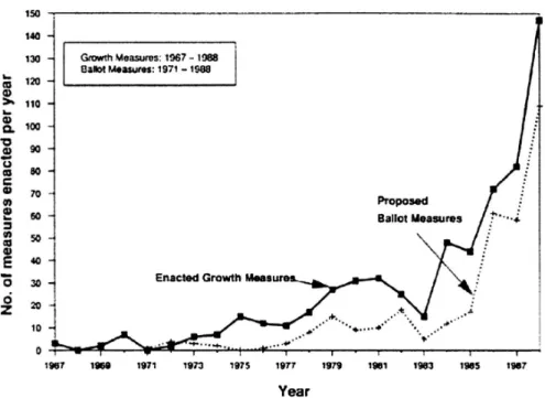
Fig. 2. Enactment of Growth Controls in California, 1967-1988

Source: Glickfeld and Levine (1992, 5) Reprinted with the permission of the Lincoln Institute of Land Policy

Fig. 3. Population in California, 1860-1990 (Census Years)

Source: Glickfeld and Levine (1992, 2) Reprinted with the permission of the Lincoln Institute of Land Policy

(8)

availability make my study confined to California of the late 1980s.

Third, for housing and population data, this study employs the 1980 Census of Population, the 1990 Census of Population and Housing, and the Population Estimates for California Counties and Cities 1970-1990. These data are provided by the U.S.

Bureau of Census and the Department of Finance of the State of California (www.dof.ca.gov).

3) Models

In order to empirically analyze the effects of local growth controls on housing construction, Equation 1 is used. This equation is the OLS regression model of homebuilding on the four different types of growth controls.

Equation 1:

LnP8890= b0+ b1LnEH90+ b2LnPG8588+ b3GC1+ b4GC2

+ b5GC3+ b6GC4+ b_7.mMSAm+ v

P8890: Average annual number of total housing building permits in each jurisdiction during 1988-90 EH90: The number of existing housing units in 1990,

which is used as a proxy for the existing housing stock in 1988

PG8588: Annual population growth rate in 1985-88 GC1: The number of population growth or housing

permit caps as of 1988

GC2: Presence or absence of urban growth boundary (1 is assigned for ‘presence’; otherwise, 0 is assigned) as of 1988

GC3: Presence or absence of adequate public facility ordinances (1 is assigned for ‘presence’; otherwise, 0 is assigned) as of 1988

GC4: The number of restrictive residential zoning regulations as of 1988

MSAm: Dummy variables indicating 24 MSAs (or PMSAs)⁶⁾; the omitted category is non-metropolitan region of California

v : Error terms

Equation 1 assumes that the business condition of

1985-1988 (represented by explanatory variables) led to issuance of building permits in 1989. The dependent variable takes the form of a 3-year average to avoid a possible bias due to the concentration of building permits in a single year. The equation uses the existing housing stock (EH90) and the annual population growth (PG8588) as control variables to extricate the impacts of the four growth controls on homebuilding. Additionally, the model employs the dummy variables of MSAs (Metropolitan Statistical Areas) to indirectly reflect the variables - housing prices, construction costs, and household income - that likely influenced homebuilding but have to be removed from Equation 1 due to multicollinearity.

The MSA dummy variables reflect other regionally varied socio-economic conditions, and likely prefer- ences of homebuilders for established and growing urban areas.

However, the OLS model (Equation 1) suffers from spatial error dependence at the queen-contiguity spatial weight matrix. This is shown by the robust Lagrange Multiplier tests (Robust LM-ERR) for spatial dependencies in Table 1. The null hypothesis that there is no spatial error dependence at the queen- contiguity spatial weight matrix has to be rejected at the 0.05 significance level. But, the null hypothesis of no spatial lag dependence at the same spatial weight matrix should not be rejected (see Robust LM-LAG of Table 1). According to Anselin (1988), spatial error dependence can occur when spatial units (here, local jurisdictions) for data aggregation do not correspond to realistic scope of a phenomenon (here, homebuilding) unfolding over space. In order to correct for this spatial autocorrelation of the OLS error terms, Equation 1 has to be converted to Equation 2, a spatial error model, which is estimated via maximum likelihood estimation.

Equation 2:

LnP8890= g0+ g1LnEH90+ g2LnPG8588+ g3GC1+ g4GC2+ g₅GC3+ g6GC4+ g_7.mMSAm+ lWv + e W: the queen-contiguity spatial weight matrix

24 m=1

S

24 m=1

S

(9)

Table 1. Equation 1: OLS and OLS White’s HCCM Estimation Variable OLS OLS - White’s HCCM Estimation

Coefficient t-value Coefficient z-value

Intercept -4.151 -13.573** -4.151 -12.326**

LnEH90 0.913 25.938** 0.913 23.364**

LnPG8588 11.728 8.260** 11.728 5.673**

GC1 0.090 1.064 0.090 1.294

GC2 0.378 3.004** 0.378 3.690**

GC3 0.068 0.702 0.068 0.735

GC4 -0.167 -2.386** -0.167 -2.380**

BAK 0.219 0.727 0.219 0.737

FRES 0.476 2.005** 0.476 2.157**

LALB -0.506 -3.224** -0.506 -3.237**

RIVSB 0.677 3.467** 0.677 3.379**

ORAN -0.542 -2.601** -0.542 -2.255**

VENT -0.035 -0.113 -0.035 -0.148

MOD 1.054 3.274** 1.054 5.796**

OAK -0.397 -1.898* -0.397 -1.453

SF -0.475 -2.340** -0.475 -2.220**

SJ -0.210 -0.857 -0.210 -1.118

SC -0.225 -0.562 -0.225 -0.607

SR 0.445 1.439 0.445 2.069**

VAL 0.786 2.813** 0.786 3.563**

SAC 0.961 4.096** 0.961 4.217**

SALI -0.022 -0.081 -0.022 -0.070

SD 0.072 0.290 0.072 0.334

SB -0.462 -1.158 -0.462 -1.177

STO 0.559 1.617 0.559 2.040**

CHIC 0.537 1.065 0.537 4.214**

REDD 0.651 1.298 0.651 1.578

VIS 0.039 0.121 0.039 0.145

YUBA 0.001 0.003 0.001 0.002

MER 0.452 1.235 0.452 1.361

SLO 0.564 1.636 0.564 2.679**

R-Square 0.7505 (F-value = 38.9950**; DF = 30, 389); Adj. R-Square = 0.7312

Regression Condition Number 22.874

Diagnostics J-B Test⁺ 5.505* (DF = 2)

B-P Test⁺⁺ 54.491** (DF = 30)

Spatial Weight 1) Up-to-50-mile 2) Up-to-40-mile 3) Up-to-25-mile 4) Queen Contiguity Contiguity Contiguity Contiguity Tests for Spatial LM-ERR⁺⁺⁺ 0.059 (DF = 1) 0.041 (DF = 1) 2.094 (DF = 1) 17.780** (DF = 1) Dependence Robust LM-ERR 0.003 (DF = 1) 0.040 (DF = 1) 2.127 (DF = 1) 7.740** (DF = 1)

LM-LAG⁺⁺⁺⁺ 0.413 (DF = 1) 0.003 (DF = 1) 0.088 (DF = 1) 10.131** (DF = 1) Robust LM-LAG 0.357 (DF = 1) 0.001 (DF = 1) 0.121 (DF = 1) 0.092 (DF = 1)

*: Significant at a = 0.1 (two-tailed); **: Significant at a = 0.05 (two-tailed); Sample Size = 420

+: Jarque-Bera test; ++: Breusch-Pagan test; +++: Lagrange multiplier test for spatial error dependence; ++++: Lagrange multiplier test for spatial lag dependence

BAK, FRES, LALB, RIVSB, ORAN, VENT, MOD, OAK, SF, SJ, SC, SR, VAL, SAC, SALI, SD, SB, STO, CHIC, REDD, VIS, YUBA, MER, and SLO: the 24 MSAs (or PMSAs)

Variable OLS OLS - White’s HCCM Estimation

Coefficient t-value Coefficient z-value

(10)

l: spatial autocorrelation coefficient of the OLS error terms, v

lWv + e: equal to v

The descriptive statistics of the variables used in Equations 1 and 2 are illustrated in Table 2. ‘Propor- tion’ in the table indicates the percentage of jurisdictions implementing each growth control out of the 420 jurisdictions. For GC1and GC4, the proportion means the percentage of jurisdictions enacting at least one sub-category belonging to each control.

The values in parentheses are the numbers of jurisdictions enacting the controls. APFOs and restrictive residential zoning have relatively higher proportions (about 30% or more), compared to population growth or housing permit caps and urban growth boundaries (more than 10% but less than 20%).

Equations 1 and 2 have the logarithmic specification of the dependent and the explanatory variables.

For the dependent variable (P8890), natural logarithm is used to avoid heteroscedasticity. In the case of the explanatory variables, the existing housing stock (EH90) and the annual population growth (PG8588), the logarithmic specification of the two variables intends to reflect potential diminishing impacts with the increases in housing stock and population growth.

Since Table 2 shows the dependent variable and the annual population growth can have negative values and 0’s for some jurisdictions, 1 is added to all the jurisdictions’ values of the two variables to allow for the logarithmic specification.

4) Results and Discussion

The results of Equation 2 are illustrated in Table 3.

My discussion focuses on the modeling results under MLE-ERR-GHET of the table. MLE-ERR- GHET corrects for the groupwise heteroscedasticity occurring between the jurisdictions of the San Francisco and Los Angeles metropolitan regions and the other jurisdictions of California as well as the spatial error dependence at the queen-contiguity spatial weight matrix. MLE-ERR means only the spatial error dependence is corrected for.

Only restrictive residential zoning (GC4) out of the four types of growth controls shows negative and significant effect on local homebuilding. On the other hand, the effects of population growth or housing permit caps (GC1) and APFOs (GC3) on local homebuilding of 1988-1990 are statistically insignificant even at the significance level of 0.1. Urban growth boundaries (GC2) demonstrate statistically significant but positive effects at 0.05. The results are interpreted in detail below.

First, population growth or housing permit caps (GC1) had no statistically significant effect on homebuilding. This is in contrast to expectation. But, considering the feature of such controls, this unexpected result is explainable. A local government can cap the annual amount of population inflow or housing building permits to slow short-period unanticipated population growth (Landis 1992). And the short-period unusual growth tends to be the basis for deter- mining the annual quota of building permits.

Table 2. Descriptive Statistics of the Variables Used in Equation 1 Variables Mean Standard Deviation Minimum Maximum Proportion

P8890 338.829 790.441 0 9,306

EH90 25,010.495 74,514.442 49 1,299,963

PG8588 0.027 0.034 -0.179 0.210

GC1 0.210 0.556 0 2 0.138 ( 58)

GC2 0.181 0.386 0 1 0.181 ( 76)

GC3 0.297 0.457 0 1 0.297 (124)

GC4 0.417 0.656 0 4 0.336 (141)

Sample Size: 420

Variables Mean Standard Deviation Minimum Maximum Proportion

(11)

Table 3. Equation 2: Spatial Error Model with Queen-Contiguity Spatial Weight Matrix Variable MLE-ERR MLE-ERR-GHET

Coefficient z-value Coefficient z-value

Intercept -4.440 -15.589** -4.442 -16.022**

LnEH90 0.936 29.341** 0.941 29.599**

LnPG8588 10.818 8.191** 10.749 8.371**

GC1 0.078 0.995 0.066 0.829

GC2 0.295 2.584** 0.294 2.636**

GC3 0.061 0.675 0.076 0.849

GC4 -0.130 -2.017** -0.120 -1.850*

BAK 0.142 0.397 0.148 0.452

FRES 0.618 2.181** 0.605 2.332**

LALB -0.579 -3.149** -0.587 -3.261**

RIVSB 0.567 2.464** 0.558 2.428**

ORAN -0.732 -2.982** -0.737 -2.981**

VENT -0.182 -0.486 -0.170 -0.443

MOD 1.209 3.140** 1.205 3.412**

OAK -0.486 -1.911* -0.494 -1.928*

SF -0.478 -1.939* -0.489 -1.972**

SJ -0.181 -0.613 -0.200 -0.666

SC -0.126 -0.271 -0.132 -0.274

SR 0.416 1.091 0.419 1.074

VAL 0.855 2.513** 0.845 2.425**

SAC 0.915 3.324** 0.911 3.602**

SALI -0.007 -0.022 -0.019 -0.063

SD 0.029 0.097 0.010 0.035

SB -0.573 -1.220 -0.582 -1.352

STO 0.584 1.454 0.585 1.583

CHIC 0.535 0.925 0.527 0.990

REDD 0.656 1.146 0.651 1.237

VIS 0.247 0.636 0.230 0.646

YUBA -0.027 -0.060 -0.026 -0.062

MER 0.585 1.358 0.587 1.482

SLO 0.468 1.118 0.470 1.226

Spatially Lagged Error Term 0.257 4.604** 0.247 4.406**

R-Square 0.7547 0.7613

Regression B-P Test 44.759** (DF = 30)

Diagnostics Spatial B-P Test 44.759** (DF = 30)

LR-GHET+ 8.129** (DF = 1)

Tests for Spatial LR-ERR++ 13.910** (DF = 1)

Dependence LM-LAG 0.085 (DF = 1)

Common Factor LR-Test 38.396 (DF = 30)

Hypothesis Test Wald Test 38.809 (DF = 30)

*: Significant at a = 0.1 (two-tailed); **: Significant at a = 0.05 (two-tailed); Sample Size = 420

+: Likelihood ratio test for groupwise heteroscedasticity; ++: Likelihood ratio test for spatial error dependence

Variable MLE-ERR MLE-ERR-GHET

Coefficient z-value Coefficient z-value

(12)

However, such rapid population growth is likely to be a deviation from average of long-term population growth. As a result, the annual quota determined by population growth or housing permit caps is rather likely to keep population growth or homebuilding at the long-term average level (Landis 1992). Given this likelihood and the continuous population growth across California (see Fig. 3), homebuilding in the jurisdictions enforcing population growth or housing permit caps, on average, will not decrease significantly, compared to other jurisdictions. As the other possible reason for the unexpected result, the fact that a relatively small number of jurisdictions enacted population growth or housing permit caps (see Table 2) could be related to the insignificant impact of GC1.

Second, the coefficient of urban growth bound- aries (GC2) is significantly positive. However, this control is assumed to inflate land prices by constrict- ing land supply (Rosen and Katz 1981; Nelson 1985;

Nelson 1986) and then reduce housing construction.

One possible reason for this counter-intuitive result is that homebuilders can circumvent land supply constraints by seeking high-density development inside the boundaries. Since any development is allowed inside the boundaries, this densification strategy works until developable land within the boundaries is depleted.⁷⁾The other possible reason is that there were likely time lags between enactment of urban growth boundaries and constrained land supply in jurisdictions. Considering that growth controls, including urban growth boundaries, main- ly spread across California in the 1980s (see Fig. 2), land supply constraints by urban growth boundaries were unlikely to take a significant effect in 1988- 1990.

Third, the regression coefficient of APFOs (GC3) is insignificant. APFOs force homebuilders to pay higher construction costs by requiring provision of sufficient public infrastructure and facilities. In addition, APFOs make homebuilders go through regulatory delays until approval is granted (Rosen and Katz 1981). Thus, APFOs are expected to have a neg-

ative effect on homebuilding. Despite this expectation, the control had no significant effect. This could be because APFOs affect homebuilders financially without restricting housing construction directly.

The ordinances allow housing construction when homebuilders supply sufficient public infrastructure to minimize costs induced by homebuilding. But, homebuilders face rising construction cost per housing unit due to the required supply of infrastructure.

Given this, in order to offset the cost increase, homebuilders can augment their housing units within the capacity of supplied public infrastructure - densification. However, this densification strategy cannot be pursued beyond the capacity of infrastructure. This may explain why the regression coefficient of APFOs is insignificantly positive.

Finally, the estimated impact of restrictive resi- dential zoning (GC4) is significantly negative. This is straightforward because the control suppresses permitted residential density on given land. Thus, such zoning constrains housing construction directly. As well, homebuilders cannot operate their businesses efficiently and fail to pursue economies of scale, given the zoning. For this reason, homebuilders face higher construction cost per housing unit and reduction of profitability. Nonetheless, homebuilders cannot increase the number of housing units on given land easily to counterbalance the rising cost. Given this unfavorable business condition, many incum- bent homebuilders are likely to become forced out of the jurisdictions implementing restrictive residential zoning. Consequently, homebuilding can be significantly constrained in the jurisdictions. In this respect, the estimated negative impact of GC4implies restrictive residential zoning likely generated a housing affordability problem.

To sum up, all other things being equal, restrictive residential zoning significantly decreased homebuilding in California jurisdictions, compared to other three types of growth controls, in the late 1980s. On the other hand, urban growth boundaries had the significant effect of accommodating housing

(13)

construction, instead of restricting homebuilding.

Population growth or housing permit caps and adequate public facility ordinances had no significant effect on homebuilding. This is possibly due to the context of California as well as the potential loop- holes of the controls.

The existing housing stock (EH90) and the annual population growth (PG8588) show significantly positive effects on housing construction. It should be noted that the estimated effect of EH90may well indi- cate a size effect. The local jurisdictions with a larger amount of housing stock (reflecting population size) likely issue more housing building permits. As regards the estimated effects of PG8588, if a certain jurisdiction experiences rapid population growth annually, the locality will face housing demand shock which will lead to a number of housing starts, all other things being equal.

4. Conclusions

This study empirically analyzes the effects of growth controls on housing construction in the local jurisdictions of California. Based on the spatial econometric modeling, the empirical analysis gains the region-wide (California-wide) generalizable results, and differentiates among the individual impacts of various growth controls on homebuilding. In addition, the analysis covers the spatial effects which have been manifested in the spatial autocorrelation of the OLS error terms. Given this, the empirical modeling of this study can contribute to filling the gaps shown in the existing works which deal with the impacts of growth controls on local housing markets, the price effects.

According to the modeling results, restrictive residential zoning shows the significantly growth-limit- ing effect in California jurisdictions. This control significantly constrained the supply of new housing in the jurisdictions than other three types of growth controls in the late 1980s. This result implies the like-

ly issue of housing affordability involved in restrictive residential zoning. On the other hand, urban growth boundaries demonstrate the effect of accommodating housing construction.

However, this paper suggests following further studies. First, in order to widen the understanding of the price effects of growth controls, other aspects of the effects (for example, the market reorientation by homebuilders towards upper segments of housing markets) have to be investigated. The constrained supply of new housing on which this paper has so far focused is only one aspect of the price effects.

Second, the impacts of growth controls enacted in neighboring jurisdictions on one locality’s housing market should be analyzed. The consideration of spatial neighbors can also encompass the spread of growth controls and the interdependence in enactment of growth controls among adjoining localities.

Thereby, it can prevent the discussion of the price effects from being one-dimensional. Finally, growth controls applied to non-residential (office or com- mercial) development have to be dealt with. This expansion can take into account possible effects of growth controls on the simultaneous interaction between population growth and employment growth that many studies have presented as an underlying process behind suburban growth (see Steinnes and Fisher 1974; Steinnes 1977; Boarnet 1994; Henry et al. 1997).

Notes

1) Growth control is different from growth management.

Whereas growth management accommodates growth in environmentally sound and fiscally effective manner (Nelson et al. 2002), growth control literally restricts growth (Landis 1992). However, both have the common goal of minimizing growth-induced costs, and cumulative effects of some growth management techniques can be similar to growth-restricting effects of growth controls (Landis 1992). Thus, this study uses growth controls and growth management interchangeably.

2) According to Mayer and Somerville (2000), regulatory

(14)

delays can include the delays for (re)zoning or subdivision approval, the negotiation over provision of on-site and off-site infrastructure (e.g., in the case of APFOs) as well as size, densities, and forms of proposed development projects, and the delays for building permits (e.g., in the case of population growth or housing permit caps).

3) However, to differentiate among the price effects is beyond the scope of this research.

4) Proposition 13 was the citizen initiative, which brought property tax assessment back to the level of 1975, permitted the annual increase in assessed value of only 2%, capped property tax rate to 1% per year, and required a super-majority approval in California state legislature for increase in the tax rate (Fulton 1993).

5) In the mid-1970s, the California State Office of Planning undertook a statewide survey which was an overview of local governments’ planning activities such as growth controls enacted and general plan elements (Elliot 1981).

The survey results were not published.

6) The definitions and constituent counties of the MSAs or PMSAs are available from the author on request.

7) In relation to this, Knaap and Nelson (1992, 40) asserts that urban growth boundary seeks to “manage the process and location of growth,” instead of restricting growth, and thus, “accommodates urban growth without permitting sprawl.”

Acknowledgement

I would like to thank Drs. Adrian Esparza, Brigitte Waldorf, and Raymond Florax for their continuous support. I also wish to acknowledge the three anonymous referees helpful comments. Particularly, two of the referees provided the constructive su- ggestions that significantly enhanced this article.

References

Ackerman, W.V., 1999, Growth control versus the growth machine in redlands, California: con- flict in urban land use, Urban Geography, 20 (2), 146-167.

Anselin, L., 1988, Spatial Econometrics: Method and Models, Dordrecht, the Netherlands,

Academic Publishers, Kulwer.

__________, 1992, SpaceStat Tutorial: A Workbook for Using SpaceStat in the Analysis of Data, Technical Software Series S-92-1, National Center for Geographic Information Analysis (NCGIA), University of California, Santa Barbara.

Boarnet, M.G., 1994, An empirical model of intrametropolitan population and employ- ment growth, Papers in Regional Science: The Journal of the RSAI, 135-152.

Byun, P. and Esparza, A.X., 2003 (forthcoming), A Revisionist model of suburbanization and sprawl: the role of political fragmentation, growth control, and Spillovers, Journal of Planning Education and Research, 23(2).

Carruthers, J.I. and Ulfarsson, G., 2002, Fragmentation and Sprawl: Evidence from interregional analysis, Growth and Change, 33, 312 - 340.

Dawkins, C.J. and Nelson, A.C., 2002, Urban containment policies and housing prices: an international comparison with implications for future research, Land Use Policy, 19, 1-12.

Dowall, D.E., 1979, The effect of land use and environmental regulations of housing costs, Policy Studies Journal, 8, 277-288.

_____________, 1984, The Suburban Squeeze: Land Conversion and Regulation in the San Francisco Bay Area, University of California Press, Berkeley, California.

Elliot, M., 1981, The impacts of growth controls regulations on housing prices in California, Journal of American Real Estate & Urban Economics Association, 9(2), 115-133.

Florax, R.J.G.M. and Nijkamp, P., 2004, Misspecification in linear spatial regression models, In K. Kempfer-Leonard (ed.), Encyclopedia of Social Measurement, Academic Press, San Diego.

Florax, R.J.G.M., Voortman, R.L., and Brouwer, J.

2002, Spatial dimensions of precision agriculture: a spatial econometric analysis of millet

(15)

yield on Sahelian coversands, Agricultural Economics, 27, 425-443.

Frieden, B.J., 1979, The new regulation comes to sub- urbia, Public Interest, 55, 15-27.

_____________, 1983, The exclusionary effects of growth controls, The Annals of the American Academy of Political and Social Science, 465, 123-135.

Fulton, W., 1993, Sliced on the cutting edge: growth management and growth control in California, in Jay M. Stein (ed.), 1993, Growth Management: the Planning Challenge of the 1990’s, Sage, Newbury Park, California, 113- 126.

Glickfeld, M. and Levine, N., 1992, Regional Growth and Local Reaction: The Enactment and Effects of Local Growth Control and Management Measures in California, Lincoln Institute of Land Policy, Cambridge, Massachusetts.

Henry, M.S., Barkley, D.L., and Bao, S., 1997, The Hinterland’s stake in metropolitan growth:

evidence from selected Southern Regions, Journal of Regional Science, 37(3), 479-501.

Janczyk, J.T. and Constance, W.C., 1980, Impacts of building moratoria on housing markets with- in a region, Growth and Change, 11(1), 11-19.

Katz, L. and Rosen, K.T., 1987, The interjurisdictional effects of growth controls on housing prices, Journal of Law & Economics, 30, 149-160.

Knaap, G. and Nelson, A.C., 1992, The Regulated Landscape: Lessons on State Land Use Planning from Oregon, Lincoln Institute of Land Policy, Cambridge, Massachusetts, 39-68.

Landis, J.D., 1986, Land regulation and the price of new housing: lesson from three California cities, Journal of the American Planning Association, 52(1), 9-21.

___________, 1992, Do growth controls work? a new assessment, Journal of the American Planning Association, 58(4), 489-508.

Levine, N., 1999, The effects of local growth controls on regional housing production and popula- tion redistribution in California, Urban

Studies, 36(12), 2047-2068.

Levy, J.M., 2000, Contemporary Urban Planning (Fifth Edition), Prentice Hall, Upper Saddle River, New Jersey.

Lillydahl, J.H. and Singell, L.D., 1987, The effects of growth management on the housing market:

a review of the theoretical and empirical evi- dence, Journal of Urban Affairs, 9(1), 63-77.

Luger, M.I. and Temkin, K., 2000, Red Tape and Housing Costs - How Regulation Affects New Residential Development, New Jersey, New Brunswick, The center for urban policy research, rutgers, The State University of New Jersey, 1-26.

Mayer, C.J. and Somerville, C.T., 2000, Land use reg- ulation and new construction, Regional Science and Urban Economics, 30, 639-662.

Nelson, A.C., 1985, Demand, segmentation, and tim- ing Effects of an urban containment program on urban fringe land values, Urban Studies, 22, 439-443.

_____________, 1986, Using land markets to evaluate urban containment progress, Journal of the American Planning Association, 52(2), 156-171.

Nelson, A.C. and Moore, T., 1993, Assessing urban growth management: the case of Portland, Oregon, the USA’s largest urban growth boundary, Land Use Policy, 10(4), 293-302.

Nelson, A.C., Pendall, R., Dawkins, C.J., and Knaap, G.J., 2002, The link between growth management and housing affordability: The acade- mic evidence, A Discussion Paper Prepared for The Brookings Institution Center on Urban and Metropolitan Policy.

Pendall, R., 2000, Local land use regulation and the Chain of exclusion, Journal of the American Planning Association, 66(2), 125-142.

Pincetl, S., 1994, The regional management of growth in California: A history of failure, International Journal of Urban and Regional Research, 18(2), 256-274.

Pollakowski, H.O. and Wachter, S.M., 1990, The

(16)

effects of land-use constraints on housing Price, Land Economics, 66(3), 315-324.

Rosen, K.T. and Katz, L.F., 1981, growth management and land use controls: The San Francisco Bay area experience, Journal of American Real Estate and Urban Economics Association, 9, 321-343.

Schwartz, S.I., Hansen, D.E., and Green, R., 1981, Suburban growth controls and the price of new housing, Journal of Environmental Economics and Managements, 8, 303-320.

_________________________________________, 1984, The effects of growth control on the produc- tion of moderate-priced housing, Land Economics, 60(1), 110-114.

Singell, L.D. and Lillydahl, J.H., 1990, An empirical examination of the effects of impact fees on the housing markets, Land Economics, 66(1), 82-92.

Skidmore, M. and Peddle, M., 1998, Do development impact fees reduce the rate of residen-

tial development?, Growth and Change, 29, 383-400.

Somerville, C.T., 1999, The industrial organization of housing supply: market activity, land supply and the size of homebuilder firms, Real Estate Economics, 27(4), 669-694.

Steinnes, D.N., 1977, Causality and intraurban loca- tion, Journal of Urban Economics, 4, 67-79.

Steinnes, D.N. and Fisher, W.D., 1974, An economet- ric model of intraurban location, Journal of Regional Science, 14(1), 65-80.

Thorson, J.A., 1997, The effect of zoning on housing construction, Journal of Housing Economics, 6, 81-91.

Zorn, P.M., Hansen, D.E., and Schwartz, S.I., 1986, Mitigating the price effects of growth con- trols: a case study of Davis, California, Land Economics, 62(1), 46-57.

Received September 15, 2003 Accepted December 11, 2003