저작자표시-비영리-변경금지 2.0 대한민국 이용자는 ... - S-Space

(1)

저작자표시-비영리-변경금지 2.0 대한민국 이용자는 아래의 조건을 따르는 경우에 한하여 자유롭게

l 이 저작물을 복제, 배포, 전송, 전시, 공연 및 방송할 수 있습니다. 다음과 같은 조건을 따라야 합니다:

l 귀하는, 이 저작물의 재이용이나 배포의 경우, 이 저작물에 적용된 이용허락조건 을 명확하게 나타내어야 합니다.

저작권법에 따른 이용자의 권리는 위의 내용에 의하여 영향을 받지 않습니다. 이것은 이용허락규약(Legal Code)을 이해하기 쉽게 요약한 것입니다.

Disclaimer

저작자표시. 귀하는 원저작자를 표시하여야 합니다.

비영리. 귀하는 이 저작물을 영리 목적으로 이용할 수 없습니다.

변경금지. 귀하는 이 저작물을 개작, 변형 또는 가공할 수 없습니다.

(2)

경영학석사 학위논문

Expectation Errors in Value/Glamour Strategies:

Evidence from the Korean Stock Market

국내 주식시장에서의 가치투자전략과 기대오류가설

2013년 2월

서울대학교 대학원

경영학과 재무 · 금융전공

최 유 진

(3)

Expectation Errors in Value/Glamour Strategies:

Evidence from the Korean Stock Market

지도교수 고 봉 찬

이 논문을 경영학석사 학위논문으로 제출함

2012년 12월

서울대학교 대학원

경영학과 재무 · 금융전공

최 유 진

최유진의 경영학석사 학위논문을 인준함

2012년 12월

위 원 장 조 재 호 (인)

부위원장 채 준 (인)

위 원 고 봉 찬 (인)

(4)

i

A BSTRACT

This paper provides evidence of expectation errors in value/glamour strategies in the Korean stock market. Under mispricing explanations, prices of glamour (value) stocks reflect systematically optimistic (pessimistic) expectations vis-à-vis the firms’ fundamentals. Grouping firms based on whether the market’s expectations (implied by B/M and C/P) are congruent or incongruent with their financial strength (implied by FSCORE), I show that the value/glamour effect is concentrated (absent) among firms with incongruent (congruent) expectations and fundamentals. The results persist after controlling for the Fama-French 3 factors, thus supporting the mispricing-based explanation for value/glamour effects.

Keywords : value, glamour, financial strength, expectation errors, mispricing Student ID : 2005-20757

(5)

ii

T ABLE OF C ONTENTS

1. Introduction ... 1

2. Research Design ... 4

2.1 Analysis framework... 4

2.2 Measurement of expectations and fundamentals ... 5

2.3 Portfolio formation and measurement of returns ... 7

2.4 Data and descriptive statistics ... 8

3. Empirical Results ... 10

3.1 Value/glamour and FSCORE portfolio returns ... 10

3.2 Value/glamour and FSCORE returns: multivariate regression ... 16

4. Robustness Tests ... 19

4.1 Fama-French 3-factor model ... 19

5. Conclusion ... 21

References ... 22

국문 초록 ... 25

(6)

iii

L IST OF T ABLES

Table 1. Composition of the FSCORE ... 6

Table 2. Descriptive statistics... 9

Table 3.1. Returns of value/glamour portfolios by B/M and FSCORE ... 12

Table 3.2. Returns of value/glamour portfolios by C/P and FSCORE ... 13

Table 4. Multivariate regression of returns to value/glamour strategies conditional on FSCORE ... 18

Table 5. Estimations of intercept and factor loadings from the F-F 3 factor model ... 20

L IST OF F IGURES

Figure 1. Portfolio distribution of expectations and fundamentals ... 5

Figure 2. Annual returns to various B/M strategies ... 15

(7)

- 1 -

1. Introduction

The strong tendency of “value” stocks, those priced cheaper relative to their fundamental values of book equity, cash flows, earnings, or dividends, to outperform their “glamour” counterparts, has been vastly evidenced in the literature (e.g. Basu 1977; Rosenberg, Reid, and Lanstein 1985; Chan, Hamao, and Lakonishok 1991; Fama and French 1992; among others).

“Value investing” has also become a widely used strategy in the investment world as a form of security analysis (Graham and Dodd 1934). However, the source of the value premium, i.e. whether the value premium is an artifact of risk or mispricing, remains unresolved to date.

Under risk-based explanations, the return differential of value stocks and glamour stocks is interpreted as compensation for additional risk. Fama and French (“F-F”, 1992, 1993) conclude that size and book-to-market (B/M) explain the cross-section of stock returns as risk factors. Vassalou (2003) contends that news related to future GDP growth (macroeconomic risk) is an important factor for explaining the cross-section of B/M and size portfolios.

Also, Petkova and Zhang (2005) report that value and glamour stocks possess different sensitivities to time-varying risks. Lettau and Wachter (2007) argue that growth and value stocks differ based on the timing of their cash flows.

Mispricing-based explanations, on the other hand, suggest that the value premium is due to expectation errors of the market. Lakonishok, Shleifer, and Vishny (1994) argue that value strategies exploit the suboptimal behavior of the typical investor. In the same vein, La Porta, Lakonishok, Shleifer, and Vishny (1997) find that one-year-ahead announcement period returns to value (glamour) firms are positive (negative). Bartov and Kim

(8)

- 2 -

(2004) report that extreme B/M ratios are due to either mis-measured accounting book values (or accruals) or mispricing, and that analysts are overly optimistic (pessimistic) about the earnings of glamour (value) stocks.

The literature on Korean data also reports a prominent value/glamour (“v/g”) effect (Kam 1997; Song 1999; Kim and Kim 2000; Kim and Kim 2001; among others); however, most Korean studies on this subject stand in support of the risk-based explanations¹.

Kim and Yun (1999) view size and B/M as proxies for risk in the cross- section of Korean stock returns, and Kim and Lim (2006) find that the F-F 3 factor model explains the value premium in Korean data. Kam and Shin (2010) argue that price momentum and financial characteristics should be considered together with B/M in value investment strategies. Lim, Baek, and Lee (2011) find that operating leverage is positively associated with B/M, and suggest that operating risk could be the source of the value premium.

The very few Korean studies from the behavioral finance approach include Chang and Kim (2007), who analyze the v/g effect in connection with technical analysis; and Kim and Byun (2010), who evidence that investor sentiment has the power to predict buy-and-hold returns in the Korean stock market.

In this study, I directly test the mispricing-based explanation for the v/g returns effect on the hypothesis that, if the prices of glamour (value) firms reflect overly optimistic (pessimistic) expectations, the v/g effect would be concentrated among firms with identifiable expectation errors and almost absent among firms without such expectation errors. In other words, the v/g

1 “The current academic climate in Korea tends to be reluctant to reflect the psychological biases of practitioners in investment management or corporate finance.

(…) Studies on Korean capital markets from the perspective of behavioral finance are limited to a few topics, and it is not easy to find studies focused on the psychological biases of investors.” (Kim and Byun 2011).

(9)

- 3 -

effect will be strongest when the market expectations are incongruent with the firms’ financial strength.

I identify expectation errors by comparing the market’s expectation (implied by the book-to-market (B/M) and cash flow-to-price (C/P) measures) against the firms’ financial fundamentals (implied by the FSCORE measure from Piotroski (2000)), and looking for congruence or incongruence therein. This two-dimensional approach follows Chang and Kim (2003) and Piotroski and So (2012), but improves on both papers.

Whereas Chang and Kim (2003) used only three measures of financial strength (operating income to sales, invested capital turnover, and interest coverage ratio), I use the FSCORE which encompasses nine measures of profitability, leverage, liquidity, and operating efficiency. Piotroski and So (2012) used only the B/M as a pricing multiple, but I add C/P to make the analysis more relevant to Korean firms.

The main findings of this study are as follows. First, the value premium exists in the Korean stock market for both B/M and C/P, even after conditioning on financial strength by FSCORE. Second, the v/g effect is most prominent among firms with incongruent expectations and fundamentals. Third, among firms with congruent expectations and fundamentals, the v/g effect in realized returns is statistically and economically close to zero. Fourth, these patterns emerge from both a portfolio approach and a regression analysis, and remain after controlling for the F-F 3 factors.

These results, consistent with the initial predictions of the study, suggest that the v/g return differential is indeed an artifact of identifiable expectation errors, thus challenging the existing explanations that are based solely on risk. I also contribute to the Korean finance literature by adding to the very

(10)

- 4 -

few existing studies stemming from the behavioral finance perspective.

2. Research Design

The purpose of this study is to examine whether the v/g effect is an artifact of market mispricing driven by expectation errors. For this I annually double-sort firm-year observations over the period of 1982 to 2011 into v/g portfolios based on the most recent B/M and C/P, and into financial strength portfolios based on the most recent FSCORE. Focusing on the congruence or incongruence of these measures, I search for predictable variation in future returns.

2.1 Analysis framework

The analysis framework for this study can be summarized in the following 3 by 3 matrix of glamour / middle / value portfolios and weak / medium / strong fundamentals portfolios, following Piotroski and So (2012).

The upper-left intersection of weak fundamentals and strong expectations (i.e. overvalued stocks), or the lower-right intersection of strong fundamentals and weak expectations (i.e. undervalued stocks) would be the portfolios where one can expect the strongest v/g effect. Conversely, the diagonal portfolios from the upper-right corner to the lower-left corner are where expectations are similar to fundamentals (i.e. neither overvalued nor undervalued stocks), thus where one can expect the weakest v/g effect.

(11)

- 5 - Figure 1

Portfolio distribution of expectations and fundamentals

2.2 Measurement of expectations and fundamentals

I use both B/M and C/P as proxies for market expectations. The B/M measure has been predominantly used in previous studies of cross-sectional stock returns and v/g strategies. The C/P measure is added in this study based on previous literature that has proved its strong relevance to the return behaviors of Korean stocks (Kam 1997; Kam 1999; Chang and Kim 2003;

among others).

To measure financial strength, I use the FSCORE from Piotroski (2000), which has also been used in Fama and French (2006). The FSCORE is a composite measure of financial trends in a firm, covering profitability, leverage, liquidity, source of funds, and operating efficiency. The FSCORE is expressed as the sum of nine binary scores (1 or 0), for the total to range from 0 to 9. The following table summarizes the composition of the FSCORE.

“Glamour”

(strong expectations)

“Middle”

(medium expectations)

“Value”

(weak expectations)

Weak

fundamentals Overvalued Potentially

overvalued

≈

Medium

fundamentals Potentially

overvalued

≈

Potentially

undervalued

Strong

fundamentals

≈

Potentially

undervalued Undervalued

(12)

- 6 - Table 1

Composition of the FSCORE

Category Definition Score

Profitability 1. ROA

Return on assets (net income before extraordinary items / beginning-of-the-year total assets)

1 if positive, 0 if otherwise 2. CFO Cash flow from operations 1 if positive, 0 if otherwise 3. △ROA Current year’s ROA – prior year’s ROA 1 if positive, 0 if otherwise 4. ACCURAL

(Net income before extraordinary items – cash flow from operations) / beginning-of-the-year total assets

1 if negative, 0 if otherwise Leverage, Liquidity, and Source of Funds

5. △LEVER

Current year’s long-term debt ratio (long-term debt / average total assets) – prior year’s long- term debt ratio

1 if negative, 0 if otherwise 6. △LIQUID Current year’s current ratio (current assets /

current liabilities) – prior year’s current ratio

1 if positive, 0 if otherwise 7. ISSUANCE Issuance of common equity 1 if none,

0 if otherwise Operating Efficiency

8. △MARGIN Current year’s gross margin ratio (gross margin / total sales) – prior year’s gross margin ratio

1 if positive, 0 if otherwise 9. △TURN Current year’s asset turnover ratio (total sales /

beginning-of-the-year total assets)

1 if positive, 0 if otherwise

(13)

- 7 -

2.3 Portfolio formation and measurement of returns

Each year, firm-year observations are allocated to value, middle, glamour portfolios and to low, mid, high FSCORE portfolios based on the prior year- end distribution of B/M, C/P, and FSCORE. Following Fama and French (1993), I classify firm-year observations with B/M ratios below the 30th percentile, between the 30th and 70th percentiles, and above the 70th percentile as “Glamour,” “Middle,” and “Value”, respectively. Following Piotroski and So (2012), firm-years with FSCORE of 0 to 3 are classified as

“low FSCORE”, 4 to 6 as “Mid FSCORE”, and 7 to 9 as “High FSCORE”.

The portfolios are formed after a four-month time period following the firms’ fiscal year-end (December for the data used in this study). Since listed firms in Korea are required to disclose annual financial information within 90 days after the fiscal year-end, I allow one additional month to cover for any late disclosures.

I measure firm-specific one- and two-year-ahead equally-weighted buy- and-hold size-adjusted returns from the beginning of the fifth month (May for the data used in this study) following the firms’ most recent fiscal year- end. Size-adjusted return is defined as the firm-specific return less the corresponding size decile portfolio return for non-financial KOSPI (Korean Composite Stock Price Index) firms.

(14)

- 8 -

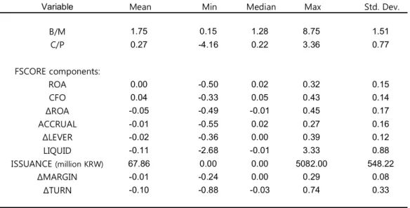
2.4 Data and descriptive statistics

The sample data for this study are all non-financial firms listed on the KOSPI market² with fiscal year-ends at December³. I include delisted firms in the sample data to reduce survivorship biases. The overall sample period is 32 years, from 1980 to 2011, for all financial data; since two years’ financial statements are required to compute the FSCORE, the time period for the return analyses is 30 years, from 1982 to 2011. Any firm-year observation lacking sufficient data to calculate the B/M, C/P, or FSCORE is deleted from the sample, yielding the final sample of 14,575 and 15,143 firm-year observations for B/M and C/P analyses, respectively. I used DataGuide of FnGuide Inc. for price-related and market data, and KisValue of NICE Information Service Co. Ltd. for accounting data. The following table presents descriptive statistics of the main variables: B/M, C/P, and FSCORE components. All variables are winsorized at the top and bottom 1 percent.

2 I exclude firms listed on the KOSDAQ (Korean Securities Dealers Automated Quotation) market, as most of the KOSDAQ-listed stocks are classified as glamour stocks (Cho, Shin, and Byun 2012) and could skew the data distribution if included in the sample.

3 Firms with fiscal year-ends at December (861) make up the vast majority (93.7%) of non-financial KOSPI firms (919) as of November 2012.

(15)

- 9 -

Variable Mean Min Median Max Std. Dev.

B/M 1.75 0.15 1.28 8.75 1.51

C/P 0.27 -4.16 0.22 3.36 0.77

FSCORE components:

ROA 0.00 -0.50 0.02 0.32 0.15

CFO 0.04 -0.33 0.05 0.43 0.14

ΔROA -0.05 -0.49 -0.01 0.45 0.17

ACCRUAL -0.01 -0.55 0.02 0.27 0.16

ΔLEVER -0.02 -0.36 0.00 0.39 0.12

LIQUID -0.11 -2.68 -0.01 3.33 0.88

ISSUANCE (million KRW) 67.86 0.00 0.00 5082.00 548.22

ΔMARGIN -0.01 -0.24 0.00 0.29 0.08

ΔTURN -0.10 -0.88 -0.03 0.74 0.33

Note: All variables are measured at the fiscal year-end prior to portfolio formation and winsorized at the top and bottom 1 percent.

Table 2 Descriptive statistics

(16)

- 10 -

3. Empirical Results

3.1 Value/glamour and FSCORE portfolio returns

Table 3.1 and Table 3.2 present one- and two-year-ahead size-adjusted returns after double-sorting firm-year observations into v/g and FSCORE portfolios, using B/M and C/P, respectively. The main findings are as follows.

First, the v/g effect persists after conditioning on the firms’ financial strength by FSCORE. V/g returns show significant differences in all the results presented: e.g. for B/M portfolios, the one-year-ahead long-short returns are 15.00%, 18.46%, and 21.85% for low, mid, and high FSCORE portfolios, respectively. The returns are even higher for two-year-ahead long- short strategies.

Second, a clear pattern emerges from the portfolio returns: in the 3 by 3 matrix of v/g and FSCORE portfolios, one can see that the returns monotonically increase as the B/M or C/P increases, and simultaneously as the FSCORE increases. This proves that B/M, C/P, and FSCORE are all positively associated with portfolio post-formation buy-and-hold size- adjusted stock returns.

Third, the v/g effect in realized returns is strongest among firms where the market expectations disagree the most with the firms’ fundamentals.

Specifically, in Panel A of Table 3.1, the highest return among the nine portfolios is found in the high FSCORE & value portfolio (18.12%), and the lowest in the low FSCORE & glamour portfolio (-9.99%). Both portfolios have extreme incongruence of expectations and fundamentals. In contrast, for portfolios where fundamentals are congruent with market expectations, the average buy-and-hold returns are closer to zero.

(17)

- 11 -

Finally, as in Piotroski and So (2012), I designate long-short investment strategies called congruent and incongruent v/g strategies. The congruent v/g strategy consists of a long position in value firms with a low FSCORE and a short position in glamour firms with a high FSCORE. The incongruent v/g strategy consists of a long position in value firms with a high FSCORE and a short position in glamour firms with a low FSCORE. The incongruent strategy generates one-year and two-year-ahead buy-and-hold size-adjusted returns that are both economically and statistically significant (28.11% and 49.71%, respectively), and higher than those of the unconditional v/g strategy (18.18% and 32.22%, respectively). Conversely, the congruent v/g strategy yields excess returns that are insignificant and much smaller (one- year and two-year-ahead size-adjusted returns of 8.74% and 13.14%, respectively).

The results for C/P (Table 3.2) are similar to those for B/M, except for the middle C/P portfolios where the returns do not increase monotonically with FSCORE. Overall, however, the results add to the evidence that the power of the C/P measure to explain stock returns is comparable to that of the B/M measure in the Korean stock market.

(18)

- 12 -

Panel A : 12-Month Return Panel B : 24-Month Return

Glamour Middle Value V-G diff. (t-statistic) Glamour Middle Value V-G diff. (t-statistic)

Unconditional -0.0713 -0.0054 0.1104 0.1818 (9.40) -0.1403 0.0013 0.1820 0.3222 (12.41)

Low FSCORE (0-3) -0.0999 -0.0581 0.0501 0.1500 (2.55) -0.1856 -0.0277 0.0402 0.2258 (3.60)

Mid FSCORE (4-6) -0.0751 -0.0054 0.1095 0.1846 (8.16) -0.1442 -0.0222 0.1881 0.3323 (10.27)

High FSCORE (7-9) -0.0373 0.0368 0.1812 0.2185 (4.05) -0.0912 0.1077 0.3116 0.4028 (6.04)

High - Low 0.0626 0.0949 0.1311 0.0943 0.1355 0.2714

(t-statistic) (1.69) (3.18) (1.85) (1.76) (2.14) (3.65)

Congruent V/G Strategy 0.0874 (1.49) 0.1314 (2.33)

Incongruent V/G Strategy 0.2811 (5.21) 0.4971 (6.89)

N Glamour Middle Value Total

Low FSCORE (0-3) 714 896 751 2,361 Mid FSCORE (4-6) 2,780 3,878 2,979 9,637 High FSCORE (7-9) 865 1,067 645 2,577 Total 4,359 5,841 4,375 14,575

Table 3.1

Returns of value/glamour portfolios by B/M and FSCORE

This table presents one-year and two-year ahead annual size-adjusted buy-and-hold returns to a B/M investment strategy, conditional upon the strength of the firm's historical fundamentals (FSCORE) for 14,575 firm-years spanning 1982 to 2011. Firm-year observations are sorted in B/M portfolios based on the preceding year's distribution of B/M realization. A firm-year observation is allocated into the Glamour, Middle, or Value portfolio if the firm’s B/M ratio is below the 30th percentile, between the 30th and 70th percentiles, or above the 70th percentile, respectively, of the preceding year’s distribution. A firm-year observation is allocated to the low FSCORE, mid FSCORE, or high FSCORE portfolio if the firm’s FSCORE is less than or equal to three, between four to seven, or greater than or equal to seven, respectively. Raw returns are defined as the firm’s twelve- or twenty-four-month buy-and-hold stock return, and size-adjusted returns are measured as raw returns minus the corresponding KOSPI size decile portfolio return. Return compounding starts at the end of four months after the most recent fiscal year-end. The Congruent V/G Strategy consists of a long position in value firms with low FSCORE and a short position in glamour firms with high FSCORE. The Incongruent V/G Strategy consists of a long position in value firms with high FSCORE and a short position in glamour firms with low FSCORE. T-statistics are shown in parentheses.

(19)

- 13 -

Panel A : 12-Month Return Panel B : 24-Month Return

Glamour Middle Value V-G diff. (t-statistic) Glamour Middle Value V-G diff. (t-statistic)

Unconditional -0.0861 -0.0141 0.1075 0.1936 (9.55) -0.1610 -0.0172 0.1686 0.3296 (11.97)

Low FSCORE (0-3) -0.1237 -0.0259 0.0767 0.2004 (2.60) -0.2084 -0.0127 0.0670 0.2754 (3.89)

Mid FSCORE (4-6) -0.0788 -0.0116 0.1022 0.1810 (7.64) -0.1506 -0.0239 0.1584 0.3090 (9.29)

High FSCORE (7-9) -0.0284 -0.0148 0.1351 0.1635 (2.90) -0.0961 0.0030 0.2411 0.3371 (5.21)

High - Low 0.0953 0.0111 0.0584 0.1123 0.0157 0.1741

(t-statistic) (1.84) (0.37) (0.73) (1.67) (0.33) (2.54)

Congruent V/G Strategy 0.1051 (1.20) 0.1631 (2.19)

Incongruent V/G Strategy 0.2588 (6.71) 0.4494 (7.43)

N Glamour Middle Value Total

Low FSCORE (0-3) 1,224 805 491 2,520 Mid FSCORE (4-6) 2,895 4,091 2,984 9,970 High FSCORE (7-9) 403 1,167 1,083 2,653 Total 4,522 6,063 4,558 15,143

Table 3.2

Returns of value/glamour portfolios by C/P and FSCORE

This table presents one-year and two-year ahead annual size-adjusted buy-and-hold returns to a C/P investment strategy, conditional upon the strength of the firm's historical fundamentals (FSCORE) for 15,143 firm-years spanning 1982 to 2011. Firm-year observations are sorted in C/P portfolios based on the preceding year's distribution of C/P realization. A firm-year observation is allocated into the Glamour, Middle, or Value portfolio if the firm’s C/P ratio is below the 30th percentile, between the 30th and 70th percentiles, or above the 70th percentile, respectively, of the preceding year’s distribution. A firm-year observation is allocated to the low FSCORE, mid FSCORE, or high FSCORE portfolio if the firm’s FSCORE is less than or equal to three, between four to seven, or greater than or equal to seven, respectively. Raw returns are defined as the firm’s twelve- or twenty-four-month buy-and-hold stock return, and size-adjusted returns are measured as raw returns minus the corresponding KOSPI size decile portfolio return. Return compounding starts at the end of four months after the most recent fiscal year-end. The Congruent V/G Strategy consists of a long position in value firms with low FSCORE and a short position in glamour firms with high FSCORE. The Incongruent V/G Strategy consists of a long position in value firms with high FSCORE and a short position in glamour firms with low FSCORE. T-statistics are shown in parentheses.

(20)

- 14 -

I also document the returns from the unconditional v/g strategy, the congruent v/g strategy, and the incongruent v/g strategy, as previously defined, for each year during the period of 1984⁴ to 2011. The key findings from the following figure are as follows. First, both the unconditional v/g strategy and the incongruent v/g strategy produce positive annual returns for most years (23 and 22, respectively, out of 28 years). Second, annual returns to the incongruent v/g strategy are larger than the unconditional v/g strategy in most years, with a time-series average annual portfolio return of 30.12%, versus 18.10% for the unconditional v/g strategy. Third, the congruent v/g strategy has the least number of annual returns that are positive (17 out of 28 years), with a time-series average annual portfolio return of 9.25%.

Additionally, to compare the returns from these v/g strategies with market conditions, I determine for each year whether the Korean stock market was a bull market, deer market, or bear market, using the annual average of the monthly returns of the KOSPI index from May of year t to April of year t + 1. The return threshold for classifying the market conditions is +/- 0.5%.

When the market is good, the incongruent v/g strategy frequently produces higher returns than both the unconditional v/g strategy and congruent v/g strategy, especially after the year 1995. When the market is flat, all three strategies show similar returns, except for the years 1991 and 1999. The year 1991 is when the market was in anticipation of the implementation of a new law⁵ requiring identity verifications of individuals when conducting any financial transaction. The year 1999 was in the midst of the Asian financial crisis, and it is interesting to see that the congruent v/g

4 The sample years 1982 and 1983 were excluded because the 1982 firms were all low FSCORE, and the 1983 firms were all low FSCORE or mid FSCORE (no high FSCORE firms), thus insufficient to construct the congruent/incongruent strategy.

5 “Act on Real Name Financial Transactions and Guarantee of Secrecy”

(21)

- 15 -

strategy has the highest return in this year. This may imply that due to the shock from such an unprecedented crisis, Korean investors became skeptical and had little expectation errors. Finally, when the market is bad, the incongruent v/g strategy consistently prevails over the unconditional v/g strategy and the congruent v/g strategy, proving the merits of the incongruent v/g strategy during bad times in particular.

This figure presents annual size-adjusted buy-and-hold returns to three investment strategies for each year of the sample from 1984 to 2011. The (+), (0), and (-) following the years denote market conditions: bull market, deer market, and bear market, respectively. Firm-year observations are sorted in B/M portfolios based on the preceding year’s distribution of B/M realizations. A firm-year observation is allocated into the Glamour, Middle, or Value portfolio if the firm’s B/M ratio is below the 30^th percentile, between the 30^th and 70^th percentiles, or above the 70^th percentile, respectively, of the preceding year’s distribution. A firm-year observation is allocated to the low FSCORE, mid FSCORE, or high FSCORE portfolio if the firm’s FSCORE is less than or equal to three, between four to seven, or greater than or equal to seven, respectively. Raw returns are defined as the firm’s 12-month buy-and-hold stock return, and size-adjusted returns are measured as raw return minus the corresponding 12-month KOSPI size decile portfolio return. Return compounding starts at the end of four months after the most recent fiscal year-end. The V/g Strategy consists of a long position in high B/M firms and a short position in low B/M firms. The Congruent V/G Strategy consists of a long position in value firms with low FSCORE and a short position in glamour firms with high FSCORE. The Incongruent V/G Strategy consists of a long position in value firms with high FSCORE and a short position in glamour firms with low FSCORE.

-50%

0%

50%

100%

150%

200%

1984 (0) 1985 (+) 1986 (+) 1987 (+) 1988 (+) 1989 (-) 1990 (0) 1991 (0) 1992 (+) 1993 (+) 1994 (0) 1995 (+) 1996 (-) 1997 (-) 1998 (+) 1999 (0) 2000 (-) 2001 (+) 2002 (-) 2003 (+) 2004 (+) 2005 (+) 2006 (+) 2007 (+) 2008 (-) 2009 (+) 2010 (+) 2011 (-)

Figure 2

Annual returns to various B/M strategies

Value/Glamour Strategy Incongruent Strategy Congruent Strategy

(22)

- 16 -

3.2 Value/glamour and FSCORE returns: multivariate regression

The previous results using the portfolio approach show significantly different return patterns across congruent and incongruent v/g portfolios.

However, this methodology is also subject to concerns that such predictability is due to omitted firm characteristics. To address these concerns, I estimate the following cross-sectional model that controls for size, momentum, and recent quarterly earnings changes, following Piotroski and So (2012):

Rit+1 = β1 Glamourit + β2 Glamourit* LowScoreit + β3 Glamourit* MidScoreit

+ β4 Middleit + β5 Middleit* LowScoreit + β6 Middleit* HighScoreit + β7 Valueit + β8 Valueit* MidScoreit + β9 Valueit* HighScoreit + β₁₀SIZE_it + β₁₁MM_it + β₁₂SUE_it + ε_it

In this regression model, the intercept term is suppressed to ensure non- collinearity among v/g classifications. SIZE is the log of market capitalization, MM (price momentum) is the preceding six-month buy-and- hold market-adjusted return, and SUE (standardized unexplained earnings) is the realized EPS minus the EPS from four quarters prior, divided by the standard deviation over the prior eight quarters.

Table 4 presents average coefficients and Fama-MacBeth Newey-West- adjusted t-statistics (to control for time-series autocorrelation) from the estimations of this model. Portfolios are formed at the end of 4 months following the fiscal year-end, at which point annual and monthly returns are matched to the most recently available financial statement data.

Value, Middle, and Glamour are indicator variables that equal one if a

(23)

- 17 -

firm’s B/M ratio is in the bottom 30%, middle 40%, and top 30% of the prior year’s distribution of B/M ratios, respectively. Similarly, LowScore, MidScore, and HighScore are indicator variables that equal one if a firm’s FSCORE is less than or equal to three, between four and six, or greater than or equal to seven, respectively. The value / middle / glamour indicator variables are interacted with the FSCORE indicator variables to capture the incongruence between expectations and fundamentals.

In this cross-sectional model specification, the coefficients on Value, Middle, and Glamour capture the fixed return effect corresponding to a specific v/g portfolio when expectations implied by firms’ B/M ratios are congruent with their fundamentals. The interaction terms capture the differential return effects of those firms subject to expectation errors within a given v/g portfolio.

Table 4 shows slightly different results from those of the portfolio analysis. The fixed return effects of glamour, middle, and value firms (e.g.

annual raw returns of 6.8%, 12.5%, and 41.7%, respectively in column (1) of Panel A) are largely consistent with the previous results, although not all coefficients are significant in the case of monthly returns. It is also noted that the differential returns conditional on FSCORE are the most significant for middle B/M firms. One can see from columns (3) that the inferences are robust to controlling for firm size (SIZE). When momentum (MM) and unexplained earnings (SUE) are added to the control variables (columns (4)), most coefficients for the annual cross-section become insignificant while they remain significant for the monthly cross-section. It also seems that the SUE subsumes a large part of the return differential, while the coefficients on the MM are insignificant. This is consistent with previous literature that reports the non-existence of momentum in the Korean stock market.

(24)

- 18 -

(1) (2) (3) (4) (1) (2) (3) (4)

Glamour 0.068 * 0.078 * 0.315 ** 0.097 0.004 0.006 0.011 ** 0.006

(1.73) (1.77) (2.04) (0.52) (1.31) (1.67) (2.57) (1.48)

Glamour * MidScore -0.012 -0.042 * -0.023 -0.001 -0.001 -0.002

(-0.73) (-1.95) (-0.91) (-0.39) (-0.79) (-1.00)

Glamour * LowScore -0.037 -0.110 -0.147 -0.007 -0.008 -0.010 **

(-0.67) (-1.37) (-1.55) (-1.23) (-1.63) (-2.06)

Middle 0.125 *** 0.124 *** 0.295 ** 0.065 0.010 *** 0.010 *** 0.015 *** 0.007 *

(3.23) (3.27) (2.50) (0.37) (3.33) (3.34) (4.02) (1.87)

Middle * LowScore -0.054 * -0.074 ** -0.071 -0.005 ** -0.005 ** -0.004 **

(-1.99) (-2.41) (-1.64) (-2.29) (-2.33) (-2.10)

Middle * HighScore 0.060 *** 0.055 ** 0.053 ** 0.004 *** 0.003 *** 0.003 *

(2.85) (2.56) (2.24) (3.26) (2.94) (1.73)

Value 0.417 ** 0.203 *** 0.312 *** 0.032 0.014 *** 0.008 0.012 ** 0.005

(2.10) (2.76) (2.92) (0.16) (3.65) (1.44) (2.28) (1.09)

Value * MidScore 0.172 0.187 0.249 0.008 ** 0.008 ** 0.007 **

(1.37) (1.39) (1.62) (2.19) (2.15) (2.67)

Value * HighScore 0.554 0.563 0.588 0.009 * 0.009 * 0.007 **

(1.22) (1.23) (1.23) (1.90) (1.96) (2.13)

Decile(SIZE) -0.036 * -0.055 * -0.001 -0.001 *

(-1.72) (-1.90) (-1.40) (-2.02)

Decile(MM) 0.018 0.000

(0.55) (0.16)

Decile(SUE) 0.067 ** 0.002 ***

(2.59) (5.97)

Rit+1 = β1 Glamourit + β2 Glamourit*LowScoreit + β3 Glamourit*MidScoreit + β4 Middleit + β5 Middleit*LowScoreit + β6 Middleit*HighScoreit

+ β7 Valueit + β8 Valueit*MidScoreit + β9 Valueit*HighScoreit + β10 SIZEit + β11 MMit + β12 SUEit + εit

Table 4

Panel A: Annual cross-sectional estimations using B/M Panel B: Monthly cross-sectional estimations using B/M Multivariate regression of returns to value/glamour strategies conditional on FSCORE

Panel A (B) presents average coefficients and Fama-MacBeth Newey-West-adjusted t-statistics from 30 annual (360 monthly) cross-sectional regressions from 1982 to 2011. For annual estimations, the dependent variable is the firm’s cumulative one-year-ahead raw return, with return compounding starting at the end of four months after the most recent fiscal year-end. For monthly estimations, monthly raw returns are matched to the most recent financial statement information available, allowing at least four months between fiscal year-end and portfolio formation. Firm-year observations are sorted in B/M portfolios based on the preceding year’s distribution of B/M realizations. A firm-year observation is allocated into the Glamour, Middle, or Value portfolio if the firm’s B/M ratio is below the 30th percentile, between the 30th and 70th percentiles, or above the 70th percentile, respectively, of the preceding year’s distribution; the indicator variables Glamour, Middle, and Value are equal to one if the firm-year corresponds to that particular B/M portfolio, zero otherwise. The indicator variables LowScore, MidScore, and HighScore are equal to one if the firm’s FSCORE is less than or equal to three, between four and six, or greater than or equal to seven, respectively. For the variables where I used deciles, SIZE is the log of market capitalization, MM is the firm’s market-adjusted return over the prior six months, and SUE is the firm’s most recent standardized unexplained earnings, calculated as realized EPS minus EPS from four quarters prior scaled by its standard deviation over the prior eight quarters. Each year, SIZE, MM, and SUE are assigned to deciles ranging from zero (lowest) to ten (highest). The intercept term is suppressed in these estimations to ensure non-collinearity among value/glamour classifications. *, **, *** denote that reported coefficients are statistically different from zero at the 10%, 5%, and 1% level of significance (two-tailed), respectively.

This table presents average coefficients from annual and monthly estimations of the following cross-sectional model for a sample of 14,575 firm-year observations from 1980 to 2011:

(25)

- 19 -

4. Robustness Tests

4.1 Fama-French 3-factor model

To further test the main hypothesis, I apply the F-F 3 factor model to the B/M investment strategies similar to those described earlier. Following Piotroski and So (2012), I designate three long-short strategies: congruent, neutral, and incongruent v/g strategies. The congruent and incongruent strategies are the same as defined in previous sections. The neutral strategy consists of a long position in value firms and a short position in glamour firms that are not allocated to either the congruent or incongruent strategies.

As such, one can expect that the risk-adjusted returns among these strategies will monotonically increase in the degree of incongruence. I estimate the following empirical asset-pricing model for each of the three strategies:

Rs,t - rft = α + β1 MKTRF + β2 SMB + β3 HML + εi,t

Rs,t is the monthly return of a given strategy in month t, rft is the risk-free rate, and MKTRF_t is the market return minus the risk-free rate. SMB_t and HML_tare the returns associated with small-minus-big firm size, and high- minus-low B/M, respectively. The KOSPI index is used as the market return and the Monetary Stabilization Bond rates as the risk-free rate. The other risk factor premiums are derived from the data of KOSPI stocks. The time period for all data is 1982-2011.

The estimation results are presented in Table 5. The most noteworthy are the alphas. After controlling for the market, size, and B/M factors, the intercepts of the three strategies monotonically increase in the degree of incongruence. For the incongruent strategy, the intercept is significant and

(26)

- 20 -

implies a 1.37% monthly excess return. For the neutral strategy, the intercept is lower, implying a monthly excess return of 0.84%. In contrast, the congruent strategy has an intercept of 0.0014 which is statistically indistinguishable from zero.

One can also see that the factor loadings on the market and size factors are decreasing in the degree of incongruence, while those on the B/M factors are increasing in incongruence, although not all statistically significant.

These patterns are largely consistent with the earlier results from the portfolio and cross-sectional regression analyses, and prove that excess returns from investment strategies with identifiable expectation errors persist even after controlling for F-F risk factors. These inferences lead one to cast significant doubt on the existing risk-based explanations for the value premium.

Intercept MKTRF SMB HML

Congruent strategy 0.0014 -0.1103 *** 0.0652 * -0.0276

(0.30) (-3.27) (1.66) (-0.62)

Neutral strategy 0.0084 * -0.1348 *** -0.0426 0.0580

(1.78) (-3.83) (-1.04) (1.24)

Incongruent strategy 0.0137 ** -0.2336 *** -0.1574 *** 0.0933

(2.09) (-4.77) (-2.76) (1.44)

This table presents estimations of the intercept and factor loadings from the following F-F 3 factor model:

Rs,t - rft = α + β1 MKTRF + β2 SMB + β3 HML + εi,t

Table 5

Estimations of intercept and factor loadings from the F-F 3 factor model

where Rs,tis the monthly return of a given strategy in month t, rftis the risk-free rate, and MKTRFtis the market return minus the risk-free rate. SMBtand HMLtare the returns associated with small-minus-big size, and high- minus-low B/M, respectively. The KOSPI index is used as the market return and the Monetary Stabilization Bond rates as the risk-free rate. The other risk factor premiums are derived from the data of KOSPI stocks. The time period for all data is 1982-2011. *, **, *** denote that reported coefficients are statistically different from zero at the 10%, 5%, and 1% level of significance (two-tailed), respectively.

(27)

- 21 -

5. Conclusion

This study examines whether a two-dimensional value investment strategy that incorporates both pricing multiples and financial fundamentals can identify expectation errors that lead to mispricing. I use the B/M and C/P as proxies for market expectations and the FSCORE as a proxy for financial strength to identify congruence or incongruence in two-dimensional value investment strategies.

The overall findings of the study provide evidence that the v/g effect is concentrated among firms with incongruent expectations and fundamentals, and almost non-existent among firms with congruent expectations and fundamentals. These results persist even after controlling for the F-F 3 factors, thus contradicting the risk-based explanations and supporting the mispricing-based explanations for v/g effects. This study also contributes to the Korean literature by making an addition to the very few existing studies stemming from the behavioral finance perspective.

(28)

- 22 -

R EFERENCES

Bartov, E., & Kim, M. (2004). Risk, mispricing, and value investing. Review of Quantitative Finance and Accounting, 23(4), 353-376.

Basu, S. (1977). Investment Performance of Common Stocks in Relation to Their Price-Earnings Ratios: A Test of the Efficient Market Hypothesis. Journal of Finance, 32(3), 663-682.

Byun, J., Shin, J., & Cho, S. (2012). The Value of a Two-Dimensional Value Investment Strategy: Evidence from the Korean Stock Market.

Emerging Markets Finance and Trade, 48(0), 58-81.

Chan, L.K.C., Hamao, Y., & Lakonishok, J. (1991). Fundamentals and stock returns in Japan. Journal of Finance, 46(5), 1739-1764.

Chang, K., & Kim, Y. (2007). Investment Performance Analysis of Value Stock and Growth Stock. Paper presented at the 2007 Summer Conference of the Korean Academic Association of Business Administration. (in Korean)

장경천, 김연권 (2007). 가치주와 성장주의 투자성과분석. 대한경영학회 2007년 하계학술발표대회 발표논문집.

Chang, Y., & Kim, C. (2003). A Value Investment Strategy: Its Performance and Sources. Korean Journal of Financial Studies, 32(2), 165-208. (in Korean)

장영광, 김종택 (2003). 한국 주식시장에서 가치투자전략의 투자성과와 그 원천. 증권학회지, 32(2), 165-208.

Cho, S., Shin, J., & Byun J. (2012). The Value of a Two-Dimensional Value Investment Strategy: Evidence from the Korean Stock Market.

Emerging Markets Finance & Trade, 48(Supplement 2), 58-81.

Fama, E.F., & French, K.R. (1992). The cross-section of expected stock returns. Journal of Finance, 47(2), 427-465.

Fama, E.F., & French, K.R. (1993). Common risk factors in the returns on stocks and bonds. Journal of Financial Economics, 33(1), 3-56.

Fama, E.F., & French, K.R. (2006). Profitability, investment and average returns. Journal of Financial Economics, 82(3), 491-518.

Graham, B., & Dodd, D. (1934). Security Analysis. New York: McGraw-Hill.

Kam, H. (1997). An Empirical Study on the Association of Fundamental Variables and Stock Returns. Korean Journal of Financial

(29)

- 23 - Management, 14(2), 21-55. (in Korean)

감형규 (1997). 기본적 변수와 주식수익률의 관계에 관한 실증적 연구. 재무관리연구, 14(2), 21-55.

Kam, H. (1999). An Empirical Study on the Performance of Contrarian Investment in Korea Stock Market. Korean Journal of Financial Management, 16(2), 157-178. (in Korean)

감형규 (1999). 한국주식시장에서의 역행투자 성과에 관한 실증적 연구. 재무관리연구, 16(2), 157-178.

Kam, H., & Shin, Y. (2010). Market Sentiment, Financial Characteristics of Firm, and the Performance of Investment Strategies in Korean Stock Market. Journal of Industrial Economics and Business, 23(1), 429- 450. (in Korean)

감형규, 신용재 (2010). 시장심리와 기업재무특성이 투자전략의 성과에 미치는 영향. 산업경제연구, 23(1), 429-450.

Kim, B., & Lee, P. (2006). An Analysis on the Long-term Performance of Value Investment Strategy in Korea. Korean Journal of Financial Studies, 35(3), 1-39. (in Korean)

김병준, 이필상 (2006). 가치투자전략의 장기적 성과 분석:

한국의 12월 결산 거래소 상장법인을 대상으로. 증권학회지, 35(3), 1-39.

Kim, K., & Byun, J. (2010). Effect of Investor Sentiment on Market Response to Stock Split Announcement. Asia-Pacific Journal of Financial Studies, 39(6), 687-719.

Kim, K., & Byun, J. (2011). Studies on Korean Capital Markets from the Perspective of Behavioral Finance. Asian Review of Financial Research, 24(3), 953-1020.

Kim, K., & Kim, Y. (2001). What Determines Expected Stock Returns in the Korean Stock Market? Korean Journal of Financial Studies, 28, 57- 85. (in Korean)

김규영, 김영빈 (2001). 한국 주식시장에서 기대수익률의 결정요인은 무엇인가? 증권학회지, 28, 57-85.

Kim, S., & Kim, J. (2000). Size, Book-to-Market, and Stock Returns. Asian Review of Financial Research, 13(2), 21-47. (in Korean)

김석진, 김지영 (2000). 기업규모와 장부가/시가 비율과 주식수익률의 관계. 재무연구, 13(2), 21-47.

Kim, S., & Yun, Y. (1999). Fundamental Variables, Macroeconomic Factors, Risk Characteristics and Equity Returns. Korean Journal of Financial Management, 16(2), 179-213. (in Korean)

(30)

- 24 -

김성표, 윤영섭 (1999). 기본적변수, 거시경제요인, 기업특성적 위험과 주식수익률. 재무관리연구, 16(2), 179-213.

La Porta, R., Lakonishok, J., Shleifer, A., & Vishny, R. (1997). Good news for value stocks: Further evidence on market efficiency. Journal of Finance, 52(2), 859-874.

Lakonishok, J., Shleifer, A., & Vishny, R. (1994). Contrarian Investment, Extrapolation, and Risk. Journal of Finance, 49(5), 1541-1578.

Lettau, M., & Wachter, J.A. (2007). Why Is Long-Horizon Equity Less Risky?

A Duration-Based Explanation of the Value Premium. Journal of Finance, 62(1), 55-92.

Lim, H., Baek, S., & Lee, Y. (2011). Investigation of the Cause of the Value Effect in Korean Stock Market: Based on Operating Leverage Hypothesis. Journal of Korean Accounting Information Association, 29(1), 133-157. (in Korean)

임형진, 백승호, 이윤원 (2011). 국내 주식시장에서 가치주 효과의 원인 분석: 영업레버리지 가설 중심. 회계정보연구, 29(1), 133-157.

Petkova, R., & Zhang, L. (2005). Is value riskier than growth? Journal of Financial Economics, 78(1), 187-202.

Piotroski, J.D. (2000). Value investing: The use of historical financial statement information to separate winners from losers. Journal of Accounting Research, 38(Supplement), 1-41.

Piotroski, J.D., & So, E.C. (2012). Identifying Expectation Errors in V/g Strategies: A Fundamental Analysis Approach. Review of Financial Studies, 25(9), 2841-2875.

Rosenberg, B., Reid, K., & Lanstein, R. (1985). Persuasive evidence of market inefficiency. Journal of Portfolio Management, 11(3), 18-28.

Song, Y. (1999). The Effects of Size and Book-to-Market Ratio on the Cross Sectional Returns. Korean Journal of Financial Studies, 24(1), 83- 103. (in Korean)

송영출 (1999). 규모와 가치비율의 수익률차이 설명력에 대한 연구. 증권학회지, 24(1), 83-103.

Vassalou, M. (2003). News related to future GDP growth as a risk factor in equity returns. Journal of Financial Economics, 68(1), 47-73.

(31)

- 25 -

국문 초록

국내 주식시장에서의 가치투자전략과 기대오류가설

최유진 경영학과 재무 · 금융전공

서울대학교 대학원

이 논문은 한국 주식시장에서의 가치주/성장주 투자전략의 성과

차이를 기대오류가설로 설명하려는 연구이다. 기대오류가설에 의하 면 성장주(가치주)의 주가 움직임은 기업의 실제 재무성과에 비하여 지나치게 낙관적인(비관적인) 시장의 기대를 반영하는 것이다. 이 논 문에서는 B/M 또는 C/P로 표현되는 시장의 기대치와 FSCORE로 표 시되는 기업의 재무건전도 간의 일치 또는 불일치 여부에 따라 포 트폴리오를 구성하여 수익률을 분석하였다. 그 결과, 가치주/성장주 효과는 시장의 기대치와 기업의 재무건전도가 불일치하는 경우에 가장 두드러지게, 일치하는 경우에 가장 약하게 나타났다. 이러한 현상은 Fama-French의 3요인을 통제한 이후에도 존재하여, 본 연구 의 결과는 가격결정오류 가설을 지지한다.

주요어 : 가치주, 성장주, 재무건전도, 기대오류, 가격결정오류 학번 : 2005-20757