저작자표시-비영리-변경금지 2.0 대한민국 이용자는 아래의 조건을 따르는 경우에 한하여 자유롭게
l 이 저작물을 복제, 배포, 전송, 전시, 공연 및 방송할 수 있습니다. 다음과 같은 조건을 따라야 합니다:
l 귀하는, 이 저작물의 재이용이나 배포의 경우, 이 저작물에 적용된 이용허락조건 을 명확하게 나타내어야 합니다.
l 저작권자로부터 별도의 허가를 받으면 이러한 조건들은 적용되지 않습니다.
저작권법에 따른 이용자의 권리는 위의 내용에 의하여 영향을 받지 않습니다. 이것은 이용허락규약(Legal Code)을 이해하기 쉽게 요약한 것입니다.
Disclaimer
저작자표시. 귀하는 원저작자를 표시하여야 합니다.
비영리. 귀하는 이 저작물을 영리 목적으로 이용할 수 없습니다.
변경금지. 귀하는 이 저작물을 개작, 변형 또는 가공할 수 없습니다.
A DISSERTATION FOR
THE DEGREE OF DOCTOR OF PHILOSOPHY
CLIMATE-SMART AGRICULTURE (CSA)-BASED ASSESSMENT OF A RICE CULTIVATION SYSTEM IN GIMJE, KOREA
핚국 김제의 벼 경작 시스템의 기후스마트농업 (Climate-Smart Agriculture) 기반의 평가
February, 2021
BY
MOHAMMAD SAMIUL AHSAN TALUCDER
INTERDISCIPLINARY PROGRAM IN
AGRICULTURAL AND FOREST METEOROLOGY
THE GRADUATE SCHOOL OF SEOUL NATIONAL UNIVERSITY
CLIMATE-SMART AGRICULTURE (CSA)-BASED ASSESSMENT OF A RICE CULTIVATION SYSTEM IN
GIMJE, KOREA
UNDER THE DIRECTION OF PROFESSOR JOON KIM, Ph.D.
SUBMITTED TO THE FACULTY OF THE GRADUATE SCHOOL OF SEOUL NATIONAL UNIVERSITY
BY
MOHAMMAD SAMIUL AHSAN TALUCDER INTERDISCIPLINARY PROGRAM IN
AGRICULTURAL AND FOREST METEOROLOGY
FEBRUARY, 2021
APPROVED AS A QUALIFIED DISSERTATION OF MOHAMMAD SAMIUL AHSAN TALUCDER
FOR THE DEGREE OF DOCTOR OF PHILOSOPHY IN AGRICULTURAL AND FOREST METEOROLOGY
BY THE COMMITTEE MEMBERS FEBRUARY, 2021
CHAIRMAN
Jin-Yong Choi, Ph.D.
VICE-CHAIRMAN
Joon Kim, Ph.D.
MEMBER
Moon-Seong Kang, Ph.D.
MEMBER
Kwang Soo Kim, Ph.D.
MEMBER
Akira Miyata, Ph.D.
i
ABSTRACT
Climate-Smart Agriculture (CSA)-Based Assessment of a Rice Cultivation System in Gimje, Korea
Mohammad Samiul Ahsan Talucder Interdisciplinary Program in Agricultural and Forest Meteorology The Graduate School of Seoul National University Food and Agriculture Organization (FAO)‟s climate-smart agriculture (CSA) challenges to avert world hunger through triple-win solutions: (1) sustainably increasing agricultural productivity and income, (2) reducing greenhouse gas (GHG) emission, and (3) building resilience to climate change. These are related to the United Nation‟s sustainable development goals (SDGs) such as SDG1 (reduce poverty), SDG2 (zero hunger), SDG12 (responsible consumption and production), SDG13 (climate action), and SDG15 (life on land). However, the paucity of appropriate (1) conceptual framework, (2) holistic indicators, and (3) quantitative measurement data hinders farmers, researchers, and policy makers from making measurable assessment of the progress and the impact of CSA.
The overarching question of this study is how a typical rice cultivation system in Korea is keeping up with the triple-win challenge of CSA. To answer this question, we have employed (1) a conceptual framework of „self-organizing hierarchical open system with visioneering‟ (SOHO-V)‟ based on complex systems perspective; (2) quantitative data from direct measurement of energy, water, carbon and information flows in and out of a rice cultivation system, and (3) appropriate metrics to assess production, efficiency, GHG fluxes, and resilience.
The study site was one of the Korean Network of Flux measurement (KoFlux) sites (i.e., GRK) located at Gimje, Korea, managed by National Academy of Agricultural Science,
ii
Rural Development Administration. Fluxes of energy, water, carbon dioxide (CO2) and methane (CH4) were directly measured using eddy-covariance technique during the growing seasons of 2011, 2012 and 2014. The production indicators include gross primary productivity (GPP), grain yield, light use efficiency (LUE), water use efficiency (WUE), crop coefficient (Kc), and carbon uptake efficiency (CUE). The GHG mitigation was assessed with indicators such as fluxes of carbon dioxide (FCO2), methane (FCH4), and nitrous oxide (FN2O).
Resilience was assessed in terms of self-organization (S), using information-theoretic approach.
The data obtained from the three growing seasons provided a wide range of contrasting environmental conditions and system states for our scrutiny. In terms of growing season averages from three years‟ monitoring, growing season length was ~122 days, solar radiation (Rs) was 1,852 MJ m-2 season-1, air temperature was 22.4°C, and precipitation (P) was 830 mm. GPP was on average 889 g C m-2, RE was 565 g C m-2, grain yield was 588 g m-2, LUE was 1.94 g C MJ-1, WUE was 1.97 g C kg H2O-1, Kc was 1.26, CUE was 1.58, FCO2 was 324 g C m-2, FCH4 was 21.1 g C m-2, FN2O was 1.65 mg N2O m-2, and SAVG was 0.40 (for half- hourly time series) and 0.09 (for daily time series). These results for GRK are mostly within the middle to upper ranges of those reported from other studies, except GHG. GRK sequestered less CO2 and emitted more CH4 and N2O than those reported from other studies.
Overall, the results of this study demonstrated that the rice cultivation system at GRK was not fulfilling the CSA‟s triple-win challenges. In fact, the competing goals and trade-offs among productivity, resilience, and GHG mitigation were found within individual years as well as between the three years, causing clashes and difficulties in achieving seamless harmony under the triple-win scenarios. The pursuit of CSA requires for stakeholders to prioritize their goals (i.e., governance) and to practice opportune interventions (i.e.,
iii
management) based on the feedback from real-time assessment of the CSA indicators (i.e., monitoring) - i.e., the purpose-driven visioneering.
The employed SOHO-V framework was useful for understanding of the complex interactions in ecological-societal systems and the CSA visioneering but difficult to use for practical application to prioritize the triad goals. An improved framework is proposed, in which economy is embedding within social systems and the UN‟s 17 SDGs are also included.
This will provide diverse stakeholders with opportunity to unifying the issues and options under one coherent vision - a healthy and sustainable world. The results from this study would facilitate a paradigm shift in agriculture from „climate-smart‟ to „climate-wise‟, which will transform ourselves from „being resilient‟ to „becoming antifragile‟ so that agriculture may gain from volatility, shocks, and uncertainties.
Key words Climate-smart agriculture, Rice, Productivity, GHG mitigation, Resilience, Self- organization, Complexity, Conceptual framework, Eddy covariance technique, Flux measurement, CSA indicator, Sustainable development goals, Paradigm shift.
Student Number: 2012-31317
iv
CONTENTS
SL. NO. TITLE PAGE
ABSTRACT i
CONTENTS iv
LIST OF TABLES vi
LIST OF FIGURES ix
LIST OF APPENDIXES xii
LIST OF ABBREVIATIONS xiii
1 INTRODUCTION 1-6
1.1 Concerns and Motive 1
1.2 Challenges in Climate-Smart Rice Farming 2
1.3 Question, Goals and Strategies 4
2. MATERIALS AND METHODS 7-26
2.1 Conceptual Framework 7
2.1.1 Self-organizing hierarchical open systems (SOHO) 7
2.1.2 Coupling of SOHO with CSA Visioneering 8
2.2 Study Site 10
2.3 Biometeorological Measurements 11
2.3.1 Theoretical Background 11
2.3.1.1 Eddy Covariance technique 12
2.3.1.2 Energy Balance 14
2.3.2 Field Measurement 15
2.4 Bio-Meteorological Data Processing 16
2.4.1 Quality control 16
2.4.2 Gap filling 16
2.5 Flux Data Processing 16
2.5.1 Raw Data Processing 16
2.5.2 Spike Detection of Fluxes 17
2.5.3 Gap-filling of Flux Data 18
2.6 Assessment of Climate-Smart Agriculture (CSA) 20
2.6.1 Indicators for productivity and efficiency 20 2.6.1.1 Gross Primary Productivity (GPP) and Grain Yield 20
2.6.1.2 Crop Coefficient (Kc) 20
2.6.1.3 Water use efficiency (WUE) 22
2.6.1.4 Light Use Efficiency (LUE) 22
2.6.2 Indicators for GHG mitigation 22
2.6.2.1 Direct Measurement of CO2 andCH4 Fluxes 23
2.6.2.2 Estimation of N2O emission 23
2.6.2.3 Carbon Uptake Efficiency (CUE) 24
2.6.3 Resilience Indicators 24
3 RESULTS 27-43
3.1 Climatic conditions 27
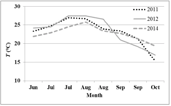
3.1.1 Air temperature 27
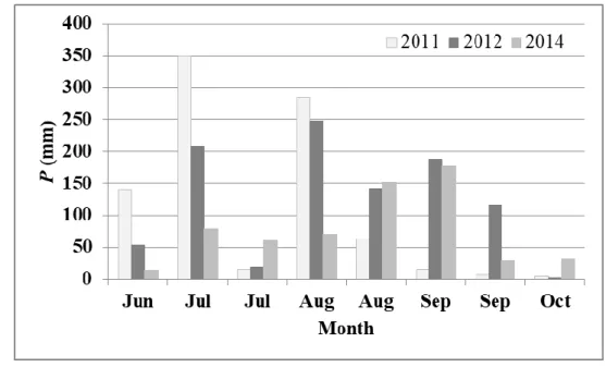
3.1.2 Precipitation 28
3.1.3 Radiation 29
3.2 Energy Balance and the Bowen Ratio 31
3.3 Assessment of Climate-Smart Agriculture (CSA) 33
3.3.1 Indicators for Productivity 33
v
SL. NO. TITLE PAGE
3.3.1.1 Gross primary productivity (GPP) 33
3.3.1.2 Evapotranspiration (ET) and crop coefficient (Kc) 34
3.3.1.3 Water use efficiency (WUE) 36
3.3.1.4 Light use efficiency (LUE) 37
3.3.2 Indicators for GHG mitigation 38
3.2.2.1 Carbon dioxide (CO2) uptake (FCO2) 38 3.2.2.2 Methane (CH4) emission (FCH4) 39 3.2.2.3 Nitrous Oxide (N2O) emission (FN2O) 40
3.3.3 Indicators for Resilience 40
4 DISCUSSION 44-59
5 SUMMARY AND CONCLUSIONS 60-63
6 SUGGESTIONS FOR FUTURE STUDY 64
7 REFERENCES 65-83
APPENDICES 83-89
ABSTRACT IN KOREAN 91-94
ACKNOWLEDGEMENT 95-97
vi
LIST OF TABLES
SL NO TITLE PAGE
Table 2.1 Transplanting, mid-summer drainage, and harvesting dates (DOY) and growing season length for Gimje rice paddy in 2011, 2012, and 2014
11
Table 3.1 Energy balance ratio (EBR), coefficient of determination (r2), and the Bowen ratio (β) from Gimje (GRK) site during the growing seasons in 2011, 2012 and 2014.
32
Table 3.2 Comparision of eddy covariance based energy balance ratio (EBR) among different rice paddy ecosystems reported in the literature
33
Table 3.3 Summary of emergence (E), self-organization (S), and complexity (C). Results are given for half-hourly time series and those from daily time series are provided in parenthesis. The subscripts GPP, FCH4, and ET represent the processes associated with gross primary production (biochemical), methane production/oxidation and transport (biogeochemical), and evapotranspiration (biophysical), respectively. The composite values (i.e., EAVG, SAVG and CAVG) were computed by taking the average of the indicators for three processes (i.e., GPP, FCH4, and ET), which are considered as overall E, S, and C indicators for the rice cultivation systems at GRK site for the growing seasons of 2011, 2012 and 2014.
42
Table 4.1 Summary of climatic conditions, phenology, and indicators for climate-smart agriculture (CSA) during the three growing seasons in 2011, 2012 and 2014 at the GRK rice cultivation site.
45
vii
SL NO TITLE PAGE
Table 4.2 Conflicts and trade-offs among the triple challenge of climate-smart agriculture (CSA) at GRK site for the growing seasons of 2011, 2012 and 2014.
47
Table 4.3 Comparison of the growing season-integrated gross primary productivity (GPP, in g C m-2) at GRK site to GPP reported from other rice paddy studies.
48
Table 4.4 Comparison of growing season-averaged light use efficiency (LUE) at GRK site to LUE reported from other rice paddy studies.
48
Table 4.5 Comparison of growing season averaged ET (mm) at GRK site to ET reported from their rice paddy studies
49
Table 4.6 Comparison of growth stage wise mean Kc of rice paddy at GRK site to Kc of rice paddy reported from ten locations of Korea. Number of days used for growth stage wise Kc estimation in this study: Kc-ini = 20; Kc-dev = 30; Kc-mid = 40; and Kc-end = 30.
50
Table 4.7 Comparison of growth stage wise mean Kc of rice paddy at GRK site to Kc of rice paddy reported from other countries.
52
Table 4.8 Comparison of the growing season averaged water use efficiency (WUE, in g C kg H2O-1) at GRK site to WUE reported from other rice paddy studies.
52
Table 4.9 Comparison of the growing season-integrated net CO2 uptake (FCO2, g C m-2) among different rice paddy ecosystems.
53
Table 4.10 Comparison of the growing season-integrated net CH4 emission (FCH4, g C m-2) among different rice paddy ecosystems.
54
viii
SL NO TITLE PAGE
Table 4.11 Comparison of the growing season-integrated N2O emission (FN2O, g N2O m-2) among different rice paddy ecosystems.
55
ix
LIST OF FIGURES
SL NO TITLE PAGE
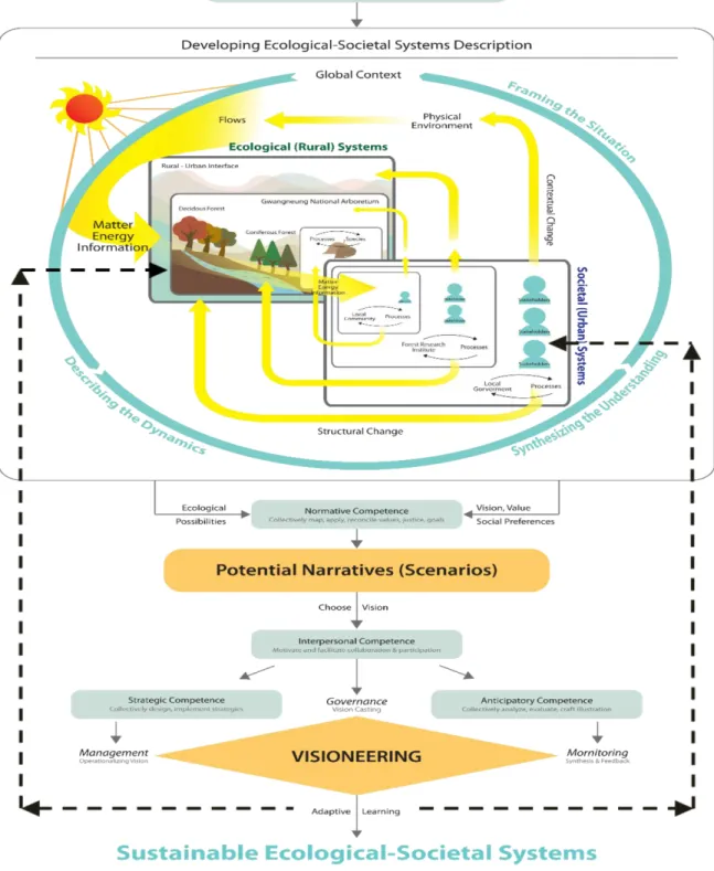
Figure 2.1 Self-organizing hierarchical open systems with visioneering (SOHO- V) framework (Kim et al., 2018). Dotted arrows describe feedback loops for adaptive learning.
9
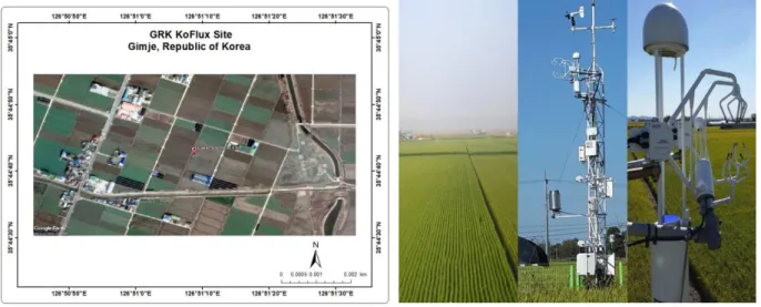
Figure 2.2 The map of the study site and the eddy covariance flux measurement tower in the rice paddy in Gimje, Korea.
10
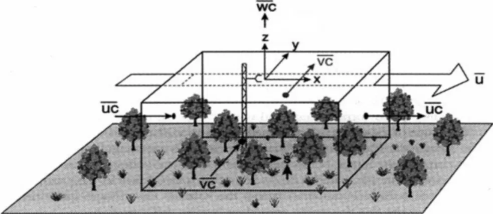
Figure 2.3 Schematic diagram of an eddy flux tower on a control volume in homogeneous flat land terrain (Finnigan et al. 2003)
12
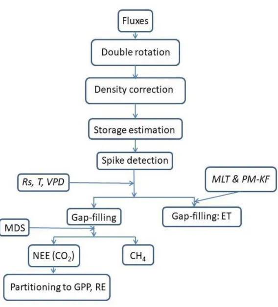
Figure 2.4 Flowchart of data processing of GRK site EC fluxes adopted from standardized KoFlux protocol (Hong et al., 2009). Here, Rs is incoming solar radiation, T is air temperature, VPD is vapor pressure deficit, MDS is marginal distribution sampling method, MLT is modified lookup table method and PM-KF is Penman-Monteith equation with Kalman filter.
19
Figure 3.1 Bi-weekly mean daily air temperature during the 2011, 2012 and 2014 growing seasons
27
Figure 3.2 Bi-weekly sum of precipitation during the 2011, 2012 and 2014 growing seasons
28
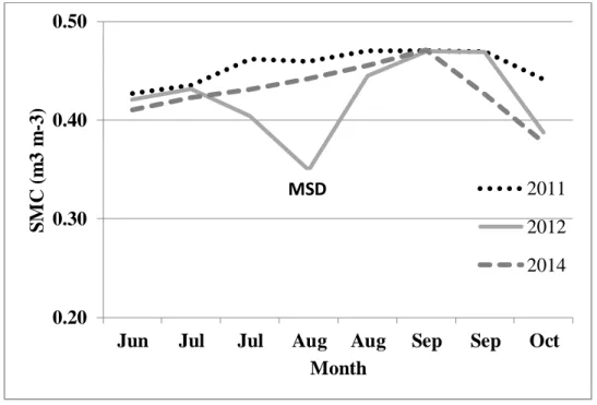
Figure 3.3 Bi-weekly average of daily soil moisture content (SMC) during the growing seasons in 2011, 2012 and 2014 at GRK site. Also shown is the mid-summer drainage (MSD) period (i.e., 21 July to 9 August 2012).
29
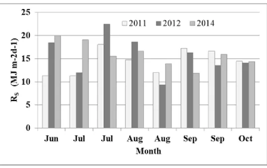
Figure 3.4 Bi-weekly averaged daily incoming solar radiation (MJ m-2 d-1) during the growing seasons in 2011, 2012 and 2014.
30
x
SL NO TITLE PAGE
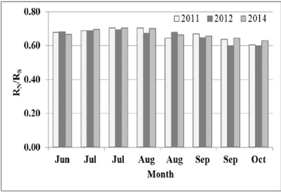
Figure 3.5 Bi-weekly averaged ratios of net radiation (Rn) to incoming solar radiation (Rs) for the growing seasons in 2011, 2012 and 2014.
31
Figure 3.6 Energy balance ratio (EBR) with regression (through the origin) using the daily integrated values of RN and + during the growing seasons in 2011, 2012 and 2014.
32
Figure 3.7 Bi-weekly sum of gross primary productivity (GPP) and ecosystem respiration (RE) during 2011, 2012 and 2014 growing seasons
34
Figure 3.8 Bi-weekly averaged daily evapotranspiration (mm d-1) during the growing seasons in 2011, 2012 and 2014.
35
Figure 3.9 Bi-weekly averaged daily crop coefficient (Kc) during the growing seasons in 2011, 2012 and 2014.
36
Figure 3.10 Bi-weekly averaged daily WUE (gC kg H2O-1d-1) during the growing seasons of 2011, 2012 and 2014.
37
Figure 3.11 Bi-weekly sum of net ecosystem exchange (NEE) during 2011, 2012 and 2014 growing seasons.
39
Figure 3.12 Bi-weekly sum of methane emission during 2011, 2012 and 2014 growing seasons.
40
Figure 4.1 Radial plot showing the relative changes (from -50 to 40%) in CSA indicators that are normalized against the mean values where FCO2 is uptake and other fluxes (FCH4 , FN2O, RE) are emission
46
Figure 4.2 CSA triad vision applied to SOHO-V framework toward sustainable agriculture
57
Figure 4.3 Ecological-Societal Systems (ESS) embedded with Doughnut 58
xi
SL NO TITLE PAGE
Economics and 17 Sustainable Development Goals (SDGs).
xii
LIST OF APPENDIXES
SL NO TITLE PAGE
A. 1 Physicochemical properties of soil at Gimje site 84 A. 2 List of Instruments at Gimje tower flux measurement
84 A. 3 Annual daily average temperature (°C) and total precipitation
(mm) of surf 243 weater station in Buan (12.4 km south-east from the Gimje study site) during 1981-2010
86
A. 4 Monthlydaily average temperature (°C) of surf 243 weater station in Buan (12.4 km South-East from the Gimje study site) during 1981-2010
87
A. 5 Monthly total precipitation (mm) of surf 243 weather station in Buan (12.4 km south-east from the Ginje study site) during 1981-2010
89
xiii
LIST OF ABBREVIATIONS C Complexity (normalized to range from 0 to 1)
CAVG Composite C
CH4 Methane
CO2 Carbon dioxide
CUE Carbon uptake efficiency E
EAVG
Emergence (normalized to range from 0 to 1) Compopsite E
EBR Energy balance ratio
EC Eddy covariance
ET Evapotranspiration (mm)
ET0 Reference evapotranspiration (mm) F
FAO
Flux (g m-2 per dayor season)
Food and Agriculture Organization (UN)
FAO-PM Food and Agriculture Organization-Penman Monteith equation
GHG Greenhouse gases
GPP Gross primary productivity (g C m-2) H Sensible heat flux (Wm-2)
IPCC The Intergovernmental Panel on Climate Change
Kc Crop coefficient
KoFlux Korean network of tower flux measurement LUE Light use efficiency
MSD Mid-season drainage
NEE N2O
Net ecosystem exchange (g C m-2 ) Nitrous oxide
P Precipitation (mm)
Pa Atmospheric pressure (kPa) Rs
RN
Incoming shortwave radiation (Wm-2) Net radiation (Wm-2)
S SAVG
Self-organization (normalized to range from 0 to 1) Composite S
SHF Soil heat flux (Wm-2)
SOHO Self-Organizing Hierarchical Open systems
SOHO-V Self-Organizing Hierarchical Open systems with Visioneering
T Air temperature (°C)
WS Wind speed (ms-1)
WUE Water use efficiency (g C Kg H2O-1 or g grain kg H2O-1)
β Bowen ratio
λE Latent heat flux (Wm-2)
1
1. INTRODUCTION
1.1 Concerns and Motive
In order to meet the world‟s future food security and sustainability needs, on one hand, food production must grow substantially to provide a certain level of food demands from population growth. On the other hand, agricultural environmental footprint also must reduce substantially (e.g., Foley et al., 2011). Current agricultural management practices have been developed in a way that demands higher resource intensity and causes significant environmental degradation. Globally, agriculture is the largest consumer (i.e. around 70 %) of all freshwater withdrawals. There is a pressing demand for a new paradigm that combines the continued development of societal system and the maintenance of the ecological system in a resilient and accommodating condition (Steffen et al., 2015). Under the framework of planetary boundary, at least four domains such as biogeochemical flows, biosphere integrity, land-system change and freshwater use are affected by agriculture, and the first two already have crossed the boundary that humanity is not supposed to cross over (http://www.stockholmresilience.org).
The increasing concerns on the role of agriculture in ensuring food security, coping with climate change, and preserving natural resources have given a birth to the vision of climate- smart agriculture (CSA) in 2010 by the United Nations Food and Agriculture Organization (FAO) (http://www.fao.org). CSA is a triple-win challenge to transforming and reorienting agricultural systems to support food security under the new realities of climate change through (1) sustainably increasing agricultural productivity and incomes, (2) reducing and/or removing greenhouse gas (GHG) emissions, where possible, and (3) adapting and building resilience to climate change. These triad goals of CSA are related to the United Nation‟s sustainable development goals (SDGs), particularly focused on reduce poverty (SDG1), zero
2
hunger (SDG2), responsible consumption and production (SDG12), climate action (SDG13), and life on land (SDG15) (http://sdgs.un.org).
The CSA initiative helps scientists, engineers, practitioners, and policy-makers to identify synergies and trade-offs among the above triad goals (e.g., Lipper et al., 2014). To further the understanding of how the implementation of CSA works in different social-ecological systems, recent progress reviews have stressed the necessities of urgent actions such as building scientific evidence and more appropriate assessment tools (e.g., Rosenstock et al., 2016). In order to ascertain the synergies and/or trade-offs among the three-fold objectives of CSA, the development of holistic indicators that are scientifically credible and relevantly integrated are imperative. However, the paucity of appropriate (1) conceptual framework, (2) holistic indicators, and (3) quantitative measurement data hinders farmers, researchers, and policy makers from making measurable assessment of the progress and the impact of CSA (e.g., Neufeldt et al., 2013; Kim et al., 2018).
1.2 Challenges in Climate-Smart Rice Farming
Rice is a leading food crop in the world (Ricepedia, n.d.). Usually, rice paddy acts as carbon sink by sequestering CO2 (Diaz et al., 2019). On the contrary, rice paddies are also one of the major sources of CH4 and its global warming potential (GWP) per unit mass is 25 times greater than that of CO2 (e.g., Miyata et al., 2000; Forster et al., 2007; Shindell et al., 2009). CH4 emission from rice paddies is expected to increase in the future due to growing demand for food, warming effect with increasing temperature, and fertilization effect with increasing CO2 concentration (e.g., Smith et al., 2007; Pereira et al., 2013; Van Groenigen et al., 2013). In addition, rice paddies are also minor sources of N2O; the GWP per unit mass is 298 times greater than that of CO2 (Forster et al., 2007; Sun et al., 2016).
3
South Korea has been striving to reinforce its agricultural production, and yet the amount of import has been increasing (KOSIS, 2015). In addition, the pressure on water resources has been substantially expanding throughout the Peninsula (e.g. Jang et al., 2010). Hence, improved water use efficiency would become an important feature under the projected water scarcity scenarios. Regarding the preparedness of Korean agriculture to be transformed to be climate-smart, there are some concerns including the lack of relevant tools to evaluate the biophysical and socio-economic impacts connected with changing climate and environmental conditions (e.g., Yoo and Kim, 2007).
Intermittent irrigation is the technique of alternately irrigating and passively or actively drying the field for several days (e.g., Keiser et al., 2002). It generally starts about two weeks after transplanting and lasts for about 10-15 weeks until the plants reach maturity. Alternate wetting and drying (AWD) is one of the technologies of intermittent irrigation. In this technique, farmers maintain the 150-mm subsurface water level threshold for re-flooding in five days interval (Lampayan et al., 2009). It is not suitable for wet season rice paddy cultivation due to monsoon. Therefore, the study site was intermittently irrigated with mid- season drainage (MSD) (Kim et al., 2016). MSD reduces the CH4 emissions since drainage affects the soil condition to change from anaerobic to aerobic, hence increasing CH4 oxidation (Nishimura et al., 2004; Wassmann et al., 2000; Sass et al., 1992). Rainfall during the MSD was reported as the major factors for causing inter-annual variations of CH4 emission from a rice paddy site at Gimje (Kim et al., 2016). Monitoring with the strength of smart farm technology could increase the effectiveness of MSD with intermittent irrigation.
Strategic and quantitative monitoring of rice paddy ecosystem is necessary to find out whether the current setting of rice paddy management is a proper configuration toward sustainable management in terms of productivity, GHG emission and system resilience to
4
climate change (e.g., Indrawati et al., 2018). It is particularly challenging to assess resilience which is associated with functionality, directionality and consequence of interaction (Nielsen and Jørgensen, 2013). From the complex systems perspective, self-organization capacity of a system has been proposed as an indicator for systems resilience (e.g. Prokopenko et al., 2009).
Currently, information-theoretic approaches attain more recognition for evaluating self- organization capacity in terms of normalize spectral entropy, for example (Zaccarelli et al., 2013; Zurlini et al., 2013). Alternatively, thermodynamics indicators have been proposed such as energy capture (ratio of incoming radiation to net radiation), energy dissipation (Lin et al., 2009; Lin et al., 2011) and thermodynamic entropy budget (Svirezhev, 2010; Brunsell et al., 2011; Cochran et al., 2016; Yang et al., 2020).
Micrometeorological eddy covariance (EC) technique provides a quantitative assessment of energy, matter, and information flows in and out of ecosystems (e.g. Yun et al., 2014;
Kang et al., 2017; Kim et al., 2018; Yang et al., 2020). The EC time series data are valuable sources not only to support model development and satellite remote sensing but also to develop useful indicators for framing the situation, describing the dynamics, and synthesizing the understanding of ecosystem-environment interactions. They can be used directly and effectively to provide quantitative and integrative indicators at ecosystem scale needed for the assessment of triple objectives of CSA.
1.3 Question, Goals and Strategies
In this study, we question, “how are rice cultivation systems in Gimje, Korea keeping up with the triple-challenge of CSA?” For the scrutiny of this assessment, we hypothesized that a typical Korean rice cultivation system is „climate-smart‟, i.e., the triad goals are not only concurrently achieved but also generally met within the levels that are from the mid to upper
5
ranges of results reported in the literature regarding productivity, GHG uptake and release, and resilience. Accordingly, a representative study site was selected from one of the Korean network of tower flux measurement (KoFlux, see Kang et al., 2018 for details) sites located at Gimje in the southwestern Korean Peninsula, which was managed by National Academy of Agricultural Science, Rural Development Administration. This study site represents one of the most typical rice farming systems in South Korea (Kim and Yeom, 2012) and the region has been designated as a „rice town” due to the role of country‟s largest and oldest artificial irrigation facilities „Byeokgolje reservoir‟ (Shim, 2009).
In order to establish quantitative database for the assessment of various CSA indicators, fluxes of energy, water, carbon dioxide (CO2) and methane (CH4) were monitored using eddy-covariance technique during the growing seasons of 2011, 2012 and 2014. The production efficiency was evaluated by examining the indicators such as gross primary productivity (GPP), ecosystem respiration (RE), grain yield, light use efficiency (LUE), water use efficiency (WUE), crop coefficient (Kc), and carbon uptake efficiency (CUE). The GHG mitigation was assessed by quantifying directly measured fluxes of carbon dioxide (FCO2) and methane (FCH4) along with indirectly estimated flux of nitrous oxide (FN2O) following the IPCC guideline (IPCC, 2006). For the resilience indicator, using information-theoretic approach, self-organization was quantified for the three most comprehensive processes in rice cultivation system (i.e., GPP, CH4 exchange, and evapotranspiration). The data obtained from the three growing seasons provided a wide range of contrasting environmental conditions and various system states for our scrutiny.
Finally, in order to streamline the processes of the CSA-based assessment, we have adopted a conceptual framework, i.e., „self-organizing hierarchical open systems (SOHO)‟
combined with „visioneering‟ feedback loops (SOHO-V) (Waltner-Toews et al., 2008; Kim
6
et al., 2018). This is a conceptual model to bring together an ecological understanding with human desire to make healthy and sustainable world, which manifests the fundamental properties of ecological-societal systems. Here, the term „hierarchical‟ means both holarchic (i.e., made up of nested levels of focus, such as the CSA triad challenges) and viewed from different and multiple perspectives (such as diverse stakeholders). Human communities as well as ecosystems are open systems and their functions and structures are organized hierarchically (e.g., Jørgensen, 2006). A nested system from multiple perspectives is a hierarchical description. The SOHO-V framework is a synthesis between traditional ways of framing both ecological problems and environmental management based on complex systems theories and the engineering of purpose-driven vision, which was used as our guide for the CSA-based assessment of rice cultivation system (see sec. 2.1 for details).
7
2. MATERIALS AND METHODS
2.1 Conceptual Framework
2.1.1 Self-organizing hierarchical open systems (SOHO)
Conceptual framework is an abstract representation, connected to the research purpose and goals that direct the collection, analysis and synthesis of data, which helps diverse practitioners and stakeholders to translate comprehensive understanding into a streamlining of priorities and strategies toward the mission and vision. In this study, we adopted a framework called „self-organizing hierarchical open systems (SOHO)‟, which provides a heuristic basis for systems thinking and a better understanding of the interactions between ecosystems and societal systems as coupled self-organizing systems. The self-organization concept implies open systems (exchanging energy, matter and information with surrounding environment) that are made up of components whose properties and behaviors are defined prior to organization itself. The term, „self‟ implies the absence of centralizing ordering or external forcing whereas „organization‟ involves a decrease in internal entropy or an increase in complexity (hence, increase in resilience) (Correia, 2006; Prokopenko et al., 2009; Kim et al., 2018).
The core assumption in the SOHO framework for the application to CSA is that a sustainable rural system maintains itself in the context of the larger ecological systems of which it is a part. The SOHO requires the integration of ecological integrity with social values and preference into a potential narrative (i.e., CSA‟s triad goals), thereby resolving a shared communal vision for climate-smart agriculture. In essence, it must involve the process of „visioneering‟ - the engineering of a clear vision (Kim and Oki, 2011). Here, engineering implies skillful direction and creative application of scientific principles and experiences to develop structures, processes, or heuristics. Visioneering stands as the cooperative triad of
8
governance (i.e., the process of strategic CSA vision casting, resolving tradeoffs and obstacles, and systematic celebration of progress), management (i.e., translating CSA vision into operation by developing and implementing priorities and strategies), and monitoring (i.e., synthesizing observations and analyses of CSA indicators into narratives, providing feedback, and promoting adaptive learning) (e.g., Boyle et al., 2001; Kim and Oki, 2011; Kim et al., 2018).
2.1.2 Coupling of SOHO with CSA Visioneering
Envisioning a climate-smart agriculture which fulfills the triple challenge is an important step.
However, without the engineering of the CSA vision, it will not stick and would remain as a daydream. Figure 2.1 represents the combined SOHO-Visioneering (SOHO-V) frame work.
Sustainability of CSA is all about maintaining the integrity of the combined ecological (i.e., rice agricultural)-societal (i.e., rural) systems. Integrity is preserved when the rice cultivation system‟s self-organizing processes are preserved, something that happens naturally if we maintain the context for self-organization in agricultural ecosystems, which, in turn, will maintain the context for the sustainability of the rural systems (e.g., Kay and Boyle, 2008;
Ash et al., 2010; Kim et al., 2018). Kim et al. (2018) further suggested that the SOHO framework should be coupled with CSA visioneering processes through feedback/feedforward loops. And these „nudged (or guided) self-organization‟ processes must be subject to first principles such as the entropy principle (as the most probable state) and the least action principle (as the most probable path/trajectory) toward sustainability.
9
Figure 2.1 Self-organizing hierarchical open systems with visioneering (SOHO-V) framework (Kim et al., 2018). Dotted arrows describe feedback loops for adaptive learning.
10
2.2 Study Site
The study site was located in the Sinyong-ri, Buryang-myeon, Gimje, Jeollabuk in the Republic of Korea (35°44´42.4˝N, 126°51´8.8˝E, and 4.2 m above m.s.l.) (Fig. 2.2). The dominant land use was cropland characterized by relatively wide plains with a moderate oceanic climate. The topography was flat and homogeneous with the prevailing wind direction from northwest. Seasonal monsoon was characterized by persistent and intensive rainy periods during the summer (i.e., „Changma‟) and frequent passes of typhoons. Soil texture was silt loam and the soil porosity was ~0.52. Rice (Oryza sativa) - winter barley (Hordeum vulgare) double crop rotation was practiced. The growing season of rice was typically from mid-June to early-October. A maximum leaf area index (LAI) was 4.4, 3.9, and 4.7 m2 m-2 in 2011, 2012, and 2014, respectively with the maximum canopy height of 1.05 m (Min et al., 2013).
Figure 2.2 The map of the study site and the eddy covariance flux measurement tower in the rice paddy in Gimje, Korea.
11
The dates of transplanting, mid-season drainage (MSD), and harvesting along with the growing season length (GSL) are summarized in Table 2.1. Thirty-day old seedlings were transplanted (5-6 seedling per hill) mechanically at a density of 30 x 15 cm with east-west planting direction. „Sindongjin‟ hybrid variety, a medium-late japonica rice cultivar, was selected mainly for their high yield potential based on performance in local yield trials (Kang et al., 2015). The nitrogen fertilizer management was barely changed. Fertilizers were applied at a rate of 110 kg N ha-1, 45 kg P2O5 ha-1 and 57 kg K2O ha-1 in total. As a basal application, 50% of N, all of P2O5 and 70% of K2O were broadcasted just prior to transplanting. The 40%
of the remaining N was applied at the tillering stage and 60% shortly after the panicle initiation stage as top dressing along with the remaining 30% of K2O. For irrigation, the water from the Bayeokgolgae reservoir was used. Flooded irrigation was carried out from early-June to mid-July, and then the paddy field was fully drained from mid-July to mid- August (i.e., mid- season drainage). After the MSD, intermittent irrigation practice was applied from mid-August to mid-September (Kim et al., 2016).
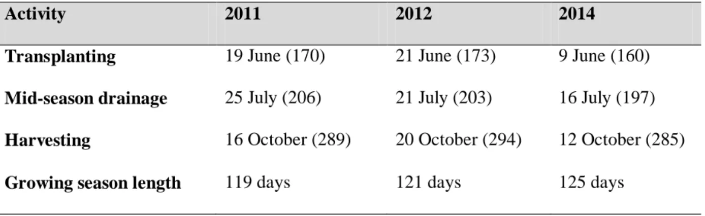
Table 2.1 Transplanting, mid-season drainage, and harvesting dates (in day of year, DOY) and growing season length (in days) for Gimje rice paddy in 2011, 2012 and 2014
Activity 2011 2012 2014
Transplanting 19 June (170) 21 June (173) 9 June (160) Mid-season drainage 25 July (206) 21 July (203) 16 July (197) Harvesting 16 October (289) 20 October (294) 12 October (285) Growing season length 119 days 121 days 125 days
2.3 Biometeorological Measurements 2.3.1 Theoretical background
12
2.3.1.1 Eddy Covariance technique
The ambient atmosphere in and above plant canopies contains turbulent motions of upward and downward moving air that transport energy and gases. The eddy covariance (EC) technique samples these turbulent motions to determine the net flux across the canopy- atmosphere interface by statistical analysis of the instantaneous vertical mass flux density ( ), using Reynolds‟ rules of averaging (Reynolds, 1895). The product of this operation is a relationship which expresses the mean flux density of a scalar averaged over some time span as the covariance between fluctuations in vertical velocity and the scalar mixing ratio ( ⁄ where is air density and is scalar density):
̅̅̅ ̅̅̅̅̅̅ (1)
where the overbars denote time averaging and the primes represent fluctuations from the mean ( ̅). Positive (or negative) covariance represents flux into (or from) the atmosphere.
Figure 2.3 Schematic diagram of an eddy flux tower on a control volume in homogeneous flat land terrain (Finnigan et al. 2003).
13
The analytical method used to measure scalar (e.g., H2O, CO2, and CH4 concentrations) also has an impact on the computation of flux covariance. In practice, scalar is measured with a non-dispersive, infrared spectrometer. This sensor does not measure mixing ratio, c. Instead, it samples molar density, (moles per unit volume). In principle, changes in molar density can occur by adding molecules to or removing them from a controlled volume or by changing the size of the controlled volume, as is done when pressure, temperature and humidity change in the atmosphere. By measuring the eddy flux covariance in terms of molar density, the net flux density of a scalar across the canopy-atmosphere interface can be written as:
̅̅̅̅̅ ̅̅̅̅̅̅ . (2)
The new term, on the right hand side of Eq. (2), is the product of the mean vertical velocity and a scalar density. The mean vertical velocity is non-zero and arises from air density fluctuations (Webb et al., 1980; Kramm et al., 1995). In practice, the magnitude of ̅ is too small (<1mms-1) to be detected by anemometry, so it is usually computed on the basis of temperature (T) and humidity density ( ) fluctuations using the Webb-Pearman-Leuning (WPL) correction (1980):
̅̅̅̅̅̅ ̅̅̅̅
̅̅̅̅̅̅̅̅̅̅ ̅̅̅̅
̅̅̅̅
̅̅̅̅̅̅̅̅̅̅ . (3)
The derivation of the above equation ignores effects of pressure fluctuations, which may be significant under high winds (Massman and Lee, 2002), and covariances between
14
temperature and pressure (Fuehrer and Friehe, 2002). It also ignores advection (Paw et al., 2000), which is important over sloping terrain.
2.3.1.2 Energy balance
Energy balance equation can be expressed as (e.g., Kang et al., 2009):
∫ ∫ ∫ , (4)
where is the net radiation, is the ground heat flux, is the energy storage, is the latent heat flux (Wm-2) and is the sensible heat flux. Daily integrated values of and are negligible (Hong and Kim, 2008). The energy balance closure was assessed using the energy balance ratio (EBR) as:
∑
∑ (5)
where the daily integrated values of and were used. The advantage of EBR is that it gives an overall evaluation of energy balance closure at longer time scales by averaging over random errors in the half-hourly measurements. A disadvantage of EBR is the potential to overlook biases in the half-hourly data, such as the tendency to overestimate positive fluxes during the day and underestimate negative fluxes at night (Mahrt, 1999). The EBR values that are differet from the unity may result from such reasons, among other factors, as mismatch of flux footprint, sampling error, instrument biases, and advection effect.
For Gimje rice paddy site, EBR was examined by linear regression (through the origin) using the daily integrated values of (H+ λE) against the daily RN during the study period. The daily integrated values of G and S were negligible. The EBR at GRK site was on average 0.96
15
(±0.09), and varied with the extent and frequency of sensible heat advection over irrigated rice paddy (i.e., positive H) mostly during mid to late afternoon period.
2.3.2 Field measurement
The EC flux measurement tower was located at the center of the paddy field to monitor energy, water vapor, CO2 and CH4 fluxes. The EC technique has the advantage of observing energy and gas fluxes over a long period with minimal disturbance to plants (e.g., Kim et al.
2000). The LI-7700 open-path CH4 analyzer (LI-COR Biosciences), the LI-7500 open-path H2O/CO2 analyzer (LI-COR Biosciences), and the CSAT3-three-dimensional sonic anemometers (Campbell Scientific Inc.) were installed at 5.2 m above the ground (see Fig. 1).
There was no vertical separation between these instruments. The horizontal separation between the LI-7700 and the CSAT3 was 0.52 m, and that between the LI-7500 and the CSAT3 was 0.43 m. The wind vectors and gas concentrations were recorded at a sampl ing rate of 10 Hz.
A rain gauge (52203 Tipping Bucket Rain Gauge, RM Young Company) was located 1 m above the ground, and a four-compnent net radiometer (CNR1, Kipp & Zonen B.V., Netherlands) was installed 2.7 m above the ground. Soil temperature and soil moisture contents at 0.05m depth were measured with thermometers (TCAV, Campbell Scientific Inc.) and tensiometers (CS616, Campbell Scientific Inc.) at 2 locations, respectively. Soil heat flux was measured with soil heat flux plates (HFP01, Hukseflux Thermal Sensors, Delft, Netherlands) which were buried at 0.05 m depth at 2 locations. The burial locations of these soil sensors were near the flux tower, which are far from a drainage channel and at a relatively low level. Such a placement led to slower drainage around the measurement area
16
than the overall conditions of the entire paddy field. A data logger (CR5000, Campbell Scientific Inc.) was used to store and compile both turbulence and meteorological data.
2.4 Bio-Meteorological Data Processing 2.4.1 Quality control
For the slow-response bio-meteorological variables, the data logger output (i.e., the 30- minutes averaged raw data without quality control) were categorized as the level 0 (L0) data.
Then, following the KoFlux data processing protocol (Hong et al., 2009, Kang et al., 2017), the L0 data were processed with quality control to produce L1 dataset.
2.4.2 Gap-filling
In order to provide seamless dataset (i.e., L2 data), the combination approach (including interpolation, mean diurnal variation, linear regression) was applied for the gap filling of the missing meteorological variables (Kang et al., 2017). These L2 data set was also used for the gap-filling of flux data measured by EC technique.
2.5 Flux Data Processing 2.5.1 Raw data processing
To improve the data quality by correcting and eliminating undesirable data, the collected flux data were examined by the quality control procedure based on the KoFlux data processing protocol (Hong et al., 2009, Kang et al., 2017). This procedure includes the coordinate rotation (double rotation; McMillen, 1988), density correction (Webb et al. 1980), storage calculation (Aubinet et al. 2001; Papale et al. 2006), Frequency response correction (Horst and Lenschow, 2009; Fratini et al., 2012), humidity correction of sonic temperature (Van
17
Dijk et al., 2004), spectroscopic correction for LI-7700 (Burba, 2013), steady state/developed turbulent conditions test (Mauder and Foken, 2011) were conducted using the EddyPro®
software (Version 5.2.1, LI-COR Biosciences). The flux and bio-meteorological data from 2011, 2012 and 2014 were used for further analysis with the exclusion of 2013 when the data availability after quality control was < 50% during the growing season.
2.5.2 Spike Detection of Fluxes
EC data are often affected by spikes due to different bio-physical and instrumental reasons.
Spike detection was conducted following Papale et al. (2006). Single point measurement storage term was added to the fluxes and then spikes were removed. The spikes in the high frequency raw data (10 Hz) are removed before the half-hourly average flux is calculated by EddyPro. However, spikes could also occur in the time series of the half hourly flux values.
KoFlux protocol was used for detecting these spikes in the half-hourly data (Hong et al., 2009) followed by Papale et al.( 2006) after some modification. The algorithm used in the matlab program to detect the spikes is based on the position of each half hourly value with respect to the values just before and after and it is applied to blocks of 28 days and separately for daytime and night-time data. Night-time data were selected according to a global radiation threshold of 20 Wm-2.
For each half-hourly data, the d value is calculated as:
(6)
and the scalar or flux value is flagged as spike if:
(
) (7) or
(
) (8)
18
where is the median of differences; median of absolute deviation ( is defined as | | and z is a threshold value.
Papale et al.( 2006) used three threshold (z) values (4, 5.5 and 7; less conservative to more conservative) to assess the effect on the data and the sensibility of the method. Seven was used as the threshold value in KoFlux protocol.
2.5.3 Gap-filling of flux data
Gap-filling was applied to processed half-hourly fluxes using the standardized KoFlux protocol (Hong et al., 2009). CO2 and CH4 fluxes were gap-filled using the marginal distribution sampling (MDS) methods, following Kang et al. (2018). In case of CO2 flux, three different nighttime CO2 flux correction (i.e., filtering and replacing) methods were applied: 1) the friction velocity (u*) filtering method, 2) light response curve (LRC) method, and 3) modified van Gorsel (mVGF) method (Kang et al., 2014; Van Gorsel et al., 2009).
The daily net ecosystem exchange (NEE), gross primary productivity (GPP) and ecosystem respiration (RE) used in this study are the averaged values from these three methods.
MDS method calculates a median fluxes under similar meteorological conditions within a time window of 14 days and replaces the missing values with the median. The intervals of the similar meteorological conditions were 50Wm−2 for the Rs, 2.5 0C for the air temperature, and 5.0 hPa for the vapor pressure deficit (VPD). If similar meteorological conditions were unavailable within the time window, its interval increased in increments of 7 days before and after the missing data point (i.e., 14-days window size) until it reached 56 days (i.e., before and after 7 days→14 days→21 days →28 days). When the missing fluxes values could not be filled in a time window of less than 56 days, Rs was exclusively used following the same approach (i.e., calculating a median of fluxes under similar Rs conditions within a time window).
19
Latent heat fluxes were gap-filled by modified lookup table method (Reichstein et al., 2005) and Penman-Monteith equation with Kalman filter whereas sensible heat fluxes were gap-filled by modified lookup table method (Reichstein et al., 2005).
Figure 2.4. Flowchart of data processing of GRK site EC fluxes adopted from standardized
KoFlux protocol (Hong et al., 2009). Here, Rs is incoming solar radiation, T is air temperature, VPD is vapor pressure deficit, MDS is marginal distribution
sampling method, MLT is modified lookup table method and PM-KF is Penman- Monteith equation with Kalman filter.
20
2.6 Assessment of Climate-Smart Agriculture (CSA) 2.6.1 Indicators for productivity and efficiency
2.6.1.1 Gross primary productivity (GPP) and grain yield
The gross primary productivity (GPP) is the total amount of organic matter produced through photosynthesis in a defined area per unit time, which represents vegetation productivity (e.g.
Gitelson et al., 2006). GPP was calculated as the sum of NEE and ecosystem respirations (RE, extrapolated from the nighttime temperature-response equation with daytime temperature) as:
GPP - RE = - NEE, (9)
where -NEE is equal to but opposite in sign to net ecosystem productivity (NEP). The nighttime ecosystem respiration was corrected using friction velocity, light response curve and modified Van Gorsel methods.
The grain yield is related to net primary productivity (NPP) which is roughly 50% of GPP (e.g. Zhang et al., 2009). In this study, the actual grain yields and GPP were used as productivity indicator. During the study period from 2011 to 2014, the rice varieties at GRK were the same, i.e., „Sindongjin‟.
2.6.1.2 Crop coefficient
Crop coefficient ( ) is a concept introduced to study the evaporative demand of the atmosphere independently of crop type, crop development, and management practices. It is the ratio of actual evapotranspiration ( ) to reference evapotranspiration ( on a daily scale:
21
, (10)
where was directly measured by the eddy covariance technique and ET0 was estimated using the globally accepted procedure - the FAO-Penmen Monteith equation (FAO-PM;
Allen et al., 1998) for humid conditions (Shuttleworth and Wallace, 1985). Here, we used instead of (RN - G) for the calculation of ET0 as:
, (11)
where ET0 is in mm d-1; is sensible heat flux (MJ m-2 d-1); λE is latent heat flux (MJ m-2 d-1);
is mean daily air temperature at 2 m height (°C); is wind speed at 2 m height (m s-1);
is saturation vapor pressure (kPa); is actual vapor pressure (kPa); is saturation vapor pressure deficit (kPa); is the slope of T-es curve (kPa °C-1); and is psychrometric constant (kPa °C-1). The wind speed at 2 m was calculated using the logarithmic wind profile equation (Rosenberg et al., 1983; Indrawati, 2015):
, (12)
where and are the mean wind speeds at elevation and , respectively. The is the zero-plane displacement and is the roughness parameter. This wind profile equation has two major assumptions: (i) the existence of neutral atmospheric stability and (ii) the availability of adequate fetch which were satisfied at this study site.
22
2.6.1.3 Water use efficiency (WUE)
Water use efficiency (WUE) at ecosystem level is defined as:
, (13)
where GPP and ET are the daily sums of half-hourly fluxes from the eddy covariance measurement (e.g. Reichstein et al., 2007; Yu et al., 2008). ET was calculated by dividing the by the latent heat of vaporization. The unit of daily GPP is in g C m-2, ET in mm, and WUE in g C kg H2O-1.
2.6.1.4 Light use efficiency (LUE)
Dry matter yield can be expressed as a function of the amount of intercepted solar radiation and the efficiency with which that radiation is converted to biomass (Monteith and Moss, 1977). The carbon exchange between the crop canopy and the atmosphere is controlled by the amount of absorbed PAR (APAR) and light use efficiency (LUE). In this study, LUE is calculated as (e.g. Gitelson and Gamon, 2015):
(14)
where is calculated from the fraction of ( ) collected from MODIS collection 6 product from a single pixel (1x1 km) around the EC tower at GRK and estimation of .
2.6.2 Indicators for GHG mitigation
23
2.6.2.1 Direct measurement of CO2 andCH4 fluxes
Measurement of GHG mitigation was assessed by the growing season-long monitoring of fluxes of CO2 and CH4 at GRK during 2011, 2012 and 2014. The time series of CO2 and CH4
fluxes were directly measured by eddy covariance techniques as described in the section 2.2 to 2.4.
2.6.2.2 Estimation of N2O emission
Nitrous oxide emissions from Gimje site were estimated following the revised 1996 IPCC guidelines for National Greenhouse gas inventories as (IPCC, 2006):
N2O emissions = Direct emissions (N2ODIRECT) + indirect emissions (N2OINDIRECT) (15) N2ODIRECT = [(FSN + FCR)x EF1FR] x 44/28, (16) N2OINDIRECT = [(N2O (G)) + (N2O (L))] x 44/28 (17)
where (i) FSN is the nitrogen (N) fertilizer applied annually to soils adjusted to account for the amount that volatilizes as NH3 and NOx [kg N ha-1], and calculated as FSN = N inputs x (1 - FracGASF) where FracGASF (volatilization factor) is 0.1 kg NH3-N/kg N2O-N; (ii) FCR is N in crop residues returned to soils [kg N ha-1], and calculated as FCR = weight of below ground part of the rice paddy (kg ha-1) x N content of the residues (0.0067 kg N kg-1 of dry biomass) where the weight of below ground part of the rice paddy was given as 87% of rice grain yield;
(iii) EF1FR is the direct emission factor for N2O emissions from N inputs to flooded rice field [kg N2O-N/kg N inputs], and the country-specific coefficient is 0.003 kg N2O-N/kg N; (iv)
N2O(G) is the indirect N2O emissions by atmospheric vaporization and estimated as N2O(G) = (FSN x FracGASF ) x EF4 where EF4 is the emission factor for N2O emissions from N
24
volatilization and re-deposition [kg N2O-N/kg NH3-N] and default value is 0.01 kg N2O-N/kg N; and (v) N2O(L) is the indirect N2O emissions by the outlet water and estimated as N2O(L) = [(FSN+FCR) x FracLEACH] x EF5 , where FracLEACH (default value = 0.3) is the fraction of N inputs losses by leaching and runoff and EF5 is the emission factor for N2O from N leaching and runoff [kg N2O-N / kg N], and the country-specific coefficient is 0.0135 kg N2O-N / kg N.
2.6.2.3 Carbon uptake efficiency
Carbon uptake efficiency (CUE) is defined as the ratio of GPP and ecosystem respiration (RE) (Indrawati et al., 2018):
(18)
where RE (in g C m-2) was estimated from EC measurement of CO2 flux. CUE describes how efficiently an ecosystem manages the carbon uptake for growth and development relative to the maintenance (e.g., Odum, 1969). CUE also represents the strength of net ecosystem carbon uptake (when CUE > 1) or release (when CUE <1). When CUE = 1, the ecosystem is carbon-neutral.
2.6.3 Resilience Indicator
Based on the SOHO framework, resilience is associated with „self-organizing capacity‟
which produces a global pattern from the interactions of the components of self-organizing systems. Such systems increase their organization in time from their own internal dynamics (Gershenson and Fernamdez, 2012). Here, information theory can be used to measure such organization (Shannon, 1948). For example, ordered/organized time series has less
25
uncertainty (i.e., low information entropy) than chaotic, disorganized time series. In other words, if information entropy is reduced, then self-organization occurs, while an increase of information entropy accompanies self-disorganization.
Complex systems are known to be equipped with stability and flexibility concurrently.
From an information-theoretic point of view, „regularity‟ ensures that useful information is maintained while „change‟ enables the systems to be flexible to explore new possibilities that are essential for adaptation and evolution. Following Lopez-Ruiz et al. (1995), complexity can be defined as the balance between change (disorder) and stability (order), for which emergence (E) and self-organization (S) can be its measure, respectively. Here, E describes emergent (new) global patterns that are not present in the system‟s components, which measures the indeterminacy a process produces as a consequence of changes in process dynamics or scale. Given a time series X (composed by a sequence of values of variable x), emergence is defined as (e.g., Santamaria-Bonfil et al., 2017):
E = −K ∑ , (19)
where K is a normalizing constant that constrains E within the range between 0 and 1 and
= P(X = x) is the probability of element i. When 1, future of x is almost certain, and E 0; then when 0, future of x is almost surely absent, so that again E 0. It is only for intermediate, less determinate values of that E remains appreciable.
Now, as resilience indicator, self-organization (S) can be seen as a reduction of entropy.
Thus, S is considered as the compliment of E, that is:
S = 1 – E, (20)