Precise Vehicle Localization Using 3D LIDAR and GPS/DR in Urban Environment

1. INTRODUCTION

Precise vehicle localization is critical for safe driving of autonomous vehicles. GPS is widely used for position recognition. However, positioning accuracy of GPS is unreliable in urban areas. In order to solve this problem, techniques for precisely recognizing the position through the combination of various sensors (GPS, IMU, camera, LIDAR, etc.) have been continuously studied.

Recently, vehicle localization techniques based on intensity map using 3D LIDAR have been extensively studied. Levinson et al. (2007), Levinson & Thrun (2010) and Hata & Wolf (2014) have presented a vehicle localization method based on road intensity maps using 3D LIDAR. Wolcott & Eustice (2014) presented a vehicle localization method based on road intensity maps using cameras. Such road intensity map based

Precise Vehicle Localization Using 3D LIDAR and GPS/DR in Urban Environment

Jun-Hyuck Im, Gyu-In Jee

Department of Electronics Engineering, Konkuk University, Seoul 05029, Korea

ABSTRACT

GPS provides the positioning solution in most areas of the world. However, the position error largely occurs in the urban area due to signal attenuation, signal blockage, and multipath. Although many studies have been carried out to solve this problem, a definite solution has not yet been proposed. Therefore, research is being conducted to solve the vehicle localization problem in the urban environment by converging sensors such as cameras and Light Detection and Ranging (LIDAR). In this paper, the precise vehicle localization using 3D LIDAR (Velodyne HDL-32E) is performed in the urban area. As there are many tall buildings in the urban area and the outer walls of urban buildings consist of planes generally perpendicular to the earth's surface, the outer wall of the building meets at a vertical corner and this vertical corner can be accurately extracted using 3D LIDAR. In this paper, we describe the vertical corner extraction method using 3D LIDAR and perform the precise localization by combining the extracted corner position and GPS/DR information. The driving test was carried out in an about 4.5 km-long section near Teheran-ro, Gangnam. The lateral and longitudinal RMS position errors were 0.146 m and 0.286 m, respectively and showed very accurate localization performance.

Keywords: precise vehicle localization, 3D LIDAR, vertical corner, GPS/DR, urban environment

vehicle localization techniques show high accuracy. However, as shown in Fig. 1, these methods have a problem in that intensity varies depending on the weather conditions of the road surface and the brightness of day and night. Particularly, the localization performance deteriorates severely in the vehicular congestion section since the road surface cannot be scanned by the LIDAR.

While there are many high buildings in urban areas that block GPS signals and the positioning accuracy of GPS is poor,

Received Feb 14, 2017 Revised Feb 20, 2017 Accepted Feb 21, 2017

†

Corresponding Author E-mail: [email protected]

Tel: +82-2-450-3070 Fax: +82-2-3437-5235 Fig. 1. Intensity map (left: wet road, right: dry road).

these high buildings can be a very good landmark for map information in the case of the precise localization method using 3D LIDAR. Map information can be represented in various forms such as 2D/3D occupancy grid map, 3D point cloud, 2D corner feature points, 2D contour (line), and 3D vertical plane. In this paper, we focused on the fact that the outer wall of the building is almost flat and perpendicular to the ground. The vertical corners of the building's exterior walls can be very good landmark information and can be extracted very precisely using the 3D LIDAR's distance information.

Also, performance deterioration does not occur in the vehicular congestion section. The present author proposed a method to utilize vertical corners of urban buildings for precise vehicle localization in a previous study (Im et al. 2016).

However, previous studies have assumed that the initial position of the vehicle is known, and the position and attitude change used in the time update of Extended Kalman Filter was calculated using Iterative Closest Point (ICP) algorithm.

ICP is not suitable for real-time implementation due to the long computation time even though ICP provides accurate position and attitude variations. In this paper, we performed vehicle precise positioning using low - cost commercial GPS/DR sensor information instead of ICP and analyzed the positioning performance after driving test near Teheran-ro, Gangnam in urban area.

This paper is organized as follows. Section 2 explains the definition and extraction of corners, and Section 3 describes the Kalman filter configuration. In Section 4, the experimental results are analyzed and in Section 5, conclusions are given.

2. CORNER DEFINITION AND EXTRACTION METHODS

2.1 Corner Definition

In general, a corner is a point or an edge that is generated

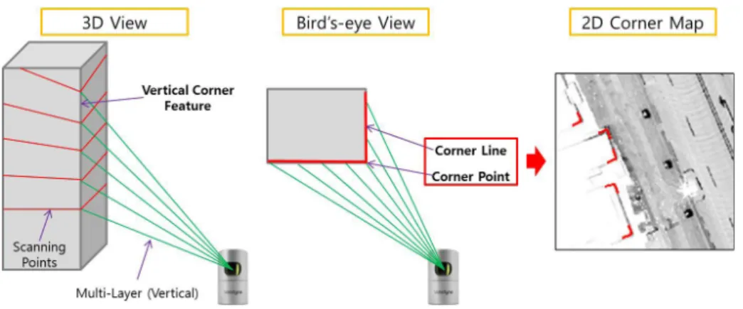
when two lines or faces meet. The exterior walls of the building are mostly almost flat and perpendicular to the ground. Therefore, there are four or more vertical corners in each building. These vertical corners are easily and accurately extracted using 3D LIDAR.

In this paper, vertical corners are projected on the ground and used as point landmarks in the 2D horizontal plane.

Fig. 2 explains the corner definition. A corner consists of one corner point and two corner lines. Fig. 3 shows the attributes of the corner feature. Corner points are represented at the 2D horizontal position in the ENU coordinate system. The corner line has directionality with respect to the corner point.

Therefore, as shown in Fig. 3, the corner line is represented by the direction angle (θ

, θ

) in the ENU coordinate system.

2.2 Corner Extraction

In this paper, Velodyne HDL-32E 3D LIDAR sensor is used and we only use the top eight layers out of the 32 layers to scan the ground because we extract the vertical corners of the building. Also, the scan data was processed for each layer.

Corner extraction requires accurate line extraction. The line extraction algorithm is presented by many researchers such as Arras & Siegwart (1997), Siadat et al. (1997), Borges

Fig. 3. Attribute of the corner feature.

Fig. 2. Corner definition.

& Aldon (2004) and Harati & Siegwart (2007). In particular, Nguyen et al. (2005) presented a paper that compares the performance of several line extraction algorithms and Iterative-End-Point-Fit (IEPF) algorithm showed the best performance and computation time. Therefore, the lines in this paper are extracted using IEPF algorithm. Fig. 4 shows the result of line extraction using IEPF algorithm. In order to easily figure out the line extraction result, it is divided into several arbitrary colors.

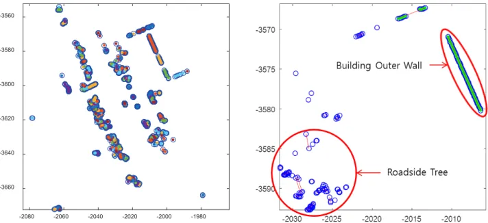
In Fig. 4, most of the extracted line components are a collection of scan points reflected by the street trees. Therefore, these outliers should be eliminated. Fig. 5 shows the reflected scan points on the exterior wall of the building and street trees. As shown in the figure, the scan points reflected by the

exterior wall of the building and street trees can be clearly distinguished. In the case of street trees, the variance in the distance between the extracted line and their scan points is much larger than the exterior wall of the building. Using these characteristics, outliers such as street trees can be easily removed. The left side of Fig. 6 is the pseudo code for outlier removal.

In the pseudo code, Var Threshold is a reference value for determining the outliers and is set considering the LIDAR distance measurement error (within about 5 cm, 95%). After outlier removal process, only the line components, which are finally determined as the outer wall of the building, are extracted as shown in the right side of Fig. 6. The corner candidates are extracted from the extracted line components

-2080 -2060 -2040 -2020 -2000 -1980

-3660 -3640 -3620 -3600 -3580 -3560

Fig. 4. Line extraction result using the IEPF algorithm.

Fig. 6. Pseudo code for outlier removal (left), line extraction result after outlier removal (right).

Fig. 5. Laser scanning points reflected by the leaves and the outer wall of

the building.

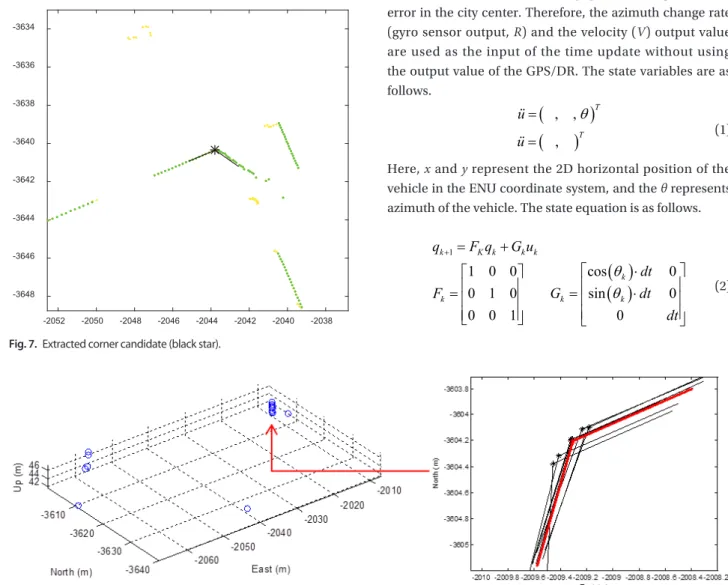
by the above-mentioned corner definition. Fig. 7 shows the extracted corner candidates.

As shown in Fig. 7, the point where a line and a line meet is extracted as a corner candidate. This process is repeated for eight layers. The left side of Fig. 8 shows the 3D position of the corner candidates extracted from the eight layers.

As shown on the left in Fig. 8, the corner candidates for each layer extracted from the same corner will have the same 2D horizontal position. Thus, when corner candidates having the same horizontal position are overlapped in certain area, the corner candidates are finally determined as corners. However, as shown on the right side of Fig. 8, the position of extracted corner candidates (black stars) for each layer for the same corner has a measurement error.

Therefore, the average value (red star) of the position of the extracted corner candidates for each layer is selected as the representative position of the finally determined corner. Fig.

9 shows the final extracted corners.

In Fig. 9, the yellow part shows the outlier such as street trees, and the green part shows the line component extracted to the outer wall of the building. The black stars represent the extracted corner candidates, and the red stars indicate the corner from which they were ultimately extracted.

3. KALMAN FILTER CONFIGURATION

3.1 Time Update

Time update uses the output value of GPS/DR. The GPS/

DR sensor uses a Micro-Infinite CruzCore DS6200 and the azimuth accuracy is within 5° of the open area. Since the 3D rotation cycle of the 3D LIDAR is set to 0.1 second, the used filter is also updated in a cycle of 0.1 second. In point landmark-based positioning, the error of position and attitude variation of the vehicle is very important. However, the GPS/DR sensor used in this paper has a large variation error in the city center. Therefore, the azimuth change rate (gyro sensor output, R) and the velocity (V) output value are used as the input of the time update without using the output value of the GPS/DR. The state variables are as follows.

( )

( )

, , ,

T T

ü ü

θ

=

= ⁽¹⁾

Here, x and y represent the 2D horizontal position of the vehicle in the ENU coordinate system, and the θ represents azimuth of the vehicle. The state equation is as follows.

( ) ( )

1

1 0 0 cos 0

0 1 0 sin 0

0 0 1 0

k K k k k

k

k k k

q F q G u

dt

F G dt

dt θ

θ

+

= +

⋅

 

 

 

 

=   =  ⋅ 

 

 

   

(2)

-2052 -2050 -2048 -2046 -2044 -2042 -2040 -2038 -3648

-3646 -3644 -3642 -3640 -3638 -3636 -3634

Fig. 7. Extracted corner candidate (black star).

Fig. 8. 3D position of corner candidates (left), corner determination result (right).

3.2 Measurement Update

Measurement update uses range and bearing measure- ments. The measurement equation is as follows.

( ) (

)

tan

i i i

i i

i

r x x y y

y y

α

x x θ

= − + −

 − 

=   −   −

(3)

Here, r

and α

are the range and bearing measurements between the vehicle and i

corner, and x

and y

are the 2D position of the i

corner in the corner map. The measurement matrix H is as follows.

-2080 -2060 -2040 -2020 -2000 -1980

-3660 -3640 -3620 -3600 -3580 -3560

Fig. 9. Corner extraction result (8 layers).

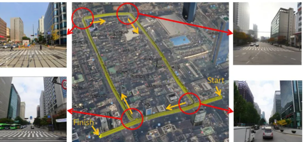
Fig. 10. Vehicle trajectory and street view (four intersections).

Fig. 11. Corner extraction result (8 layers).

( )

( ) ( )

( )

( ) ( )

( )

( ) ( ) ( )

( ) ( )

( )

( ) ( )

( )

( ) ( )

( )

( ) ( ) ( )

( ) ( )

1 1

2 2 2 2

1 1 1 1

1 1

2 2 2 2

1 1 1 1

2 2 2 2

2 2 2 2

0 1

0 1

n n

n n n n

n n

n n n n

x x y y

x x y y x x y y

y y x x

x x y y x x y y

H

x x y y

x x y y x x y y

y y x x

x x y y x x y y

− − − −

 

 

− + − − + −

 

 

− − −

 − 

 − + − − + − 

 

 

=  

− − − −

 

 − + − − + − 

 

 − − − 

 − 

 − + − − + − 

 

   (4)

4. EXPERIMENTAL RESULTS

As shown in Fig. 10, the driving experiment was conducted near Teheran-ro, Gangnam in the central city area. The distance traveled from the start point to the end point was 4.5 km, the maximum speed was about 80 km/h, and the average speed was about 60 km/h. The positioning error was calculated based on the results of the vehicle driving trajectory optimization (GraphSLAM) used for the corner map generation. Fig. 11 shows the corner-based localization error.

As shown in Fig. 11, the corner map-based localization technique has a much better positioning accuracy than the GPS/DR and RTK/INS results. The lateral RMS error is 0.146 m and the longitudinal RMS error is 0.286 m. The maximum error is about 1.1 m in the lateral direction and about 1.9 m in the longitudinal direction. In case of GPS/DR, errors occur very much in the urban environment.

Even if the rate of change of the azimuth angle of the sensor and the velocity output value are used, there is a case where the very large change of the position error occurs.

If there are no or few corners to be extracted at this case, a large position error will occur. Fig. 11 generally shows position accuracy within about 20 cm, but this is the case where large position error often occurs. Fig. 12 shows the number of extracted corners.

In Figs. 11 and 12, as shown in the epoch of 500, 1300, and 2400, when the number of extracted corners is very small, a position error of 1 m or more occurs. Fig. 13 shows Probability Density Function (PDF) and RMS error for each extracted corner number. As shown in the figure, when two or more corners are seen, both lateral and longitudinal RMS errors are limited to within about 20 cm. In this case, the RMS error is relatively large when the number of extracted corners is 6. However, as shown in the PDF, when the number of corners extracted is 6 or more, it is difficult to evaluate the valid result because the number of corners is very small.

The reason why the longitudinal position error is larger in Fig. 11 than in the lateral direction is related to the layout of the building. Buildings where corners can be extracted are always on both sides of the road and there is no building in the driving direction of the vehicle, which is the longitudinal direction. For this reason, the Dilution of Precision of the corner measurement is worse than the lateral direction.

If additional landmark information, which is located in the driving direction of the vehicle, such as traffic lights and road signs, is used, longitudinal performance can be improved.

5. CONCLUSIONS

Recently, the positional accuracy required for autonomous

driving is within 50 cm in the lateral direction. This is a

Fig. 12. Number of the extracted corners. Fig. 13. PDF and 2D RMS error for each number of extracted corners.

minimum requirement for vehicles not to leave the lane, considering lane width and vehicle width. In this paper, vertical corners are extracted using 3D LIDAR in the urban area, and precise vehicle localization is conducted by combining with GPS/DR. Experimental results show that the accuracy of position is within 25 cm in lateral direction and within 50 cm in longitudinal direction in over 95% range.

Thus, the positioning method proposed in this paper satisfies the position accuracy required for autonomous driving.

However, the reliability of 95% should be further improved.

As mentioned above, a large position error occurs in a region where the number of extracted corners is very small.

Therefore, localization performance can be greatly improved if corner extraction performance is improved or other additional landmarks that can complement the corner are used at the same time. Later, these studies should be conducted continuously.

REFERENCES

Arras, K. O. & Siegwart, R. 1997, Feature extraction and scene interpretation for map-based navigation and map building, in Proceedings of the Symposium on Intelligent Systems and Advanced Manufacturing, Pittsburgh, PA, USA, 14-17, October 1997.

Borges, G. A. & Aldon, M. J. 2004, Line extraction in 2D range images for mobile robotics, Journal of Intelligent and Robotic Systems, 40, 267-297. http://dx.doi.org/10.1023/

B:JINT.0000038945.55712.65

Harati, A. & Siegwart, R. 2007, A new approach to segmentation of 2D range scans into linear regions, in Proceedings of the IEEE/RSJ International Conference on Intelligent Robots and Systems, San Diego, CA, USA, 29 October–2 November 2007. http://dx.doi.org/10.1109/IROS.2007.4399499 Hata, A. & Wolf, D. 2014, Road marking detection using LIDAR

reflective intensity data and its application to vehicle localization, 2014 IEEE 17th International Conference on Intelligent Transportation Systems (ITSC), Qingdao, China, 8-11 Oct. 2014. http://dx.doi.org/10.1109/

ITSC.2014.6957753

Im, J.-H., Im, S.-H., & Jee, G.-I. 2016, Vertical corner feature based precise vehicle localization using 3D LIDAR in urban area, Sensors, 16, E1268. http://dx.doi.org/10.3390/

s16081268

Levinson, J., Montemerlo, M., & Thrun, S. 2007, Map-based precision vehicle localization in urban environments, In Robotics Science and Systems III, June 27-30, 2007, Georgia Institute of Technology, Atlanta, Georgia, USA.

http://dx.doi.org/10.15607/RSS.2007.III.016

Levinson, J. & Thrun, S. 2010, Robust vehicle localization in urban environments using probabilistic maps, in Proceedings of the 2010 IEEE International Conference on Robotics and Automations, Anchorage, Convention District, May 3-8, 2010, Anchorage, Alaska, USA. http://

dx.doi.org/10.1109/ROBOT.2010.5509700

Nguyen, V., Martinelli, A., Tomatis, N., & Siegwart, R. 2005, A comparison of line extraction algorithms using 2D laser rangefinder for indoor mobile robotics, in Proceedings of the IEEE/RSJ International Conference on Intelligent Robots and Systems, Edmonton, AB, Canada, 2-6, August 2005. http://dx.doi.org/10.1109/

IROS.2005.1545234

Siadat, A., Kaske, A., Klausmann, S., Dufaut, M., & Husson, R. 1997, An optimized segmentation method for a 2D laser-scanner applied to mobile robot navigation, in Proceedings of the 3rd IFAC Symposium on Intelligent Components and Instruments for Control Applications, Annecy, France, 9-11, June 1997.

Wolcott, R. W. & Eustice, R. M. 2014, Visual localization within LIDAR maps for automated urban driving, in Proceedings of the 2014 IEEE/RSJ International Conference on Intelligent Robots and Systems (IROS 2014), Chicago, IL, USA, 14-18 Sept. 2014. http://dx.doi.

org/10.1109/IROS.2014.6942558

Jun-Hyuck Im received the B.S. degree in the Dept. of Electronic Engineering from Hongik University in 2008 and the M.S. degree from Konkuk University in 2011. He is currently pursuing the Ph.D. degree in Electronic Engineering in Konkuk University. His research interests include LIDAR-based localization, Map building, SLAM, Autonomous vehicle, Loran-C signal processing, Indoor positioning, GPS, INS.

Gyu-In Jee received Ph.D in System

Engineering from Case Western Reserve

University in 1989. He is a professor of

E l e c t ro n i c s Eng i n e e r i ng o f Ko n ku k

University. His research interests include

Indoor GPS positioning, Software GNSS

receiver, GPS/Galileo baseband FPGA

design, Anti-Jamming, Autonomous vehicle, Map-based

localization, Map building.