IEG 환경지질연구정보센터

1. Introcuction

A variety of techniques for analyzing remotely- sensed images have been developed for applications that include characterizing and classifying land cover.

Statistical pattern recognition techniques have conventionally been used in classification of remotely- sensed imagery (Zenzo et al., 1987; Mohn et al., 1987).

Signal variability through time results in artificial

expressions of differences in land-cover types that often cause classification errors. The development of multi- temporal techniques has been primarily motivated by the difficulty in discriminating between surface material types based on the spectral signatures at a single point in time. A typical approach for the analysis of temporal patterns in remote sensing data involves the visual examination of temporal sequence of individual pixels using “temporal profile” plotting (Tucker, et al., 1990;

Classification of Land Cover on Korean Peninsula Using Multi-temporal NOAA AVHRR Imagery

Sang-Hoon Lee

Department of Industrial Engineering, Kyungwon University

Abstract :Multi-temporal approaches using sequential data acquired over multiple years are essential for satisfactory discrimination between many land-cover classes whose signatures exhibit seasonal trends.

At any particular time, the response of several classes may be indistinguishable. A harmonic model that can represent seasonal variability is characterized by four components: mean level, frequency, phase and amplitude. The trigonometric components of the harmonic function inherently contain temporal information about changes in land-cover characteristics. Using the estimates which are obtained from sequential images through spectral analysis, seasonal periodicity can be incorporates into multi-temporal classification. The Normalized Difference Vegetation Index (NDVI) was computed for one week composites of the Advanced Very High Resolution Radiometer (AVHRR) imagery over the Korean peninsula for 1996 ~ 2000 using a dynamic technique. Land-cover types were then classified both with the estimated harmonic components using an unsupervised classification approach based on a hierarchical clustering algorithm. The results of the classification using the harmonic components show that the new approach is potentially very effective for identifying land-cover types by the analysis of its multi-temporal behavior.

Key Words :Harmonic Model, Multi-temporal Classification, AVHRR, NDVI, Land-cover Type.

Received 14 August 2003; Accepted 25 September 2003.

Teng, 1990). Multi-temporal features have also been exploited through knowledge-based approaches (Carlotto, 1985; Goldberg et al., 1983). However, statistical approaches for the analysis of multi-temporal remotely-sensed images remain largely unexplored, and few are designed to preserve the sequence contains abundant, useful information. Multi-temporal techniques involve concatenating multiple spectral data sets separated in time and analyzing the combined spectral- temporal feature vector. One difficulty in the analysis of multi-temporal image data is encountered with evaluating the temporal trends simultaneously with spatial trends. This problem can be resolved by reducing the dimensionality of the temporal data. One approach is to use a transformation of multi-temporal data through the determination of the area-under-the-curve or the integral of the temporal profile curve (Tucker, et al., 1990). In this transformation, temporal trends in the processes are summarized by a single number that is associated with the temporal accumulation measure. The purpose of this paper is to present observational evidence to show the potential for improved information extraction with a sequence of multi-temporal data using an alternative approach.

Reflectance data from the Advanced Very High Resolution Radiometer (AVHRR) that is deployed on the NOAA-n series of polar orbiting meteorological satellites are obtainable globally on a daily basis and have been shown to have considerable potential for large scale land vegetation studies. Analyses of the relations between AVHRR spectral measurements and vegetation related phenomena have been exceptionally successful and have encouraged great interest in the AVHRR sensor as a global vegetation observatory (Horvath et al., 1982; Townsend and Tucker, 1984). The unique capacity of the AVHRR to resolve landscape at reasonable spatial resolution and high temporal resolution is critical to this type of research. Multi- temporal remotely-sensed data have been shown to be

successful in monitoring seasonal trends in phonological processes.

Multi-spectral reflectance data have been transformed and combined into various vegetation indices to minimize the variability due to external factors (Tarpley et al., 1984). The most commonly used vegetation index is the normalized difference vegetation index (NDVI), and the NDVI versus time profile then reflects each vegetation’s seasonal development history. The shape of the seasonal profile may be used to evaluate the type of vegetation cover on the basis of the magnitude and shape of the curve. Sampson (1993) proposed two indices that characterize the shape of a curve developed from a seasonal profile of NDVI. These indices complement the area-under-the-curve integral index by reflecting the time in seasonal profile and the range of the NDVI values in the temporal sequence. In this paper, an alternative approach is investigated to characterize the temporal profile of NDVI processes as a means of reducing dimensionality for multi-temporal classification. The seasonality of vegetation types can be represented with a harmonic model characterized by four components: mean level, frequency, amplitude and phase. The parameterization provides physically interpretable values with which to characterize the seasonal development of a vegetated pixel. The mean index represents the average level of spectral intensity over the whole period that the data were compiled. The periodicity of ground cover response is described by the frequency index. The amplitude and phase indices are reference values associated with the growing season of a particular vegetation type. One reflects the range of variation in the spectral measurements and the other the initiation time for the peak of growth. Using the estimates that are obtained through spectral analysis of a sequence of composite imagery, seasonal periodicity can be incorporated into multi-temporal classification. The resulting classification based on these components reflects different sources of temporal variation.

In this study, the NDVI images were computed for NOAA AVHRR imagery over the Korean Peninsula for 1996 and 2000, and the harmonic components from this five-year sequence were estimated via spectral analysis.

Land-cover types were then classified using the multistage classification algorithm that makes use of hierarchical clustering (Lee, 2001). Section II describes a harmonic model for multi-temporal data. The classification algorithm is briefly reviewed in Sections III. Section IV contains the results of the spectral analysis and classification. Conclusions are presented in Section V.

2. Harmonic Model

Many physical processes that have been sensed and displayed in the image from the land exhibit temporal variation with seasonal periodicity. The process of seasonality can be represented with a harmonic model shoes components are assumed to be only due to target characteristics. Thus, the temporal sequence of each pixel has a harmonic model according to the seasonal profile of its class.

A sample image is considered as a set of n pixels and the intensity process can be represented in the form

Xt= mm_t(c) + ee_t

(1) m

mt(c) = {mt,c(i)= ac(i)+ Rc(i)sin(wc(i)t + qc(i)), i ∈In} where In= {1, 2,…, n} is a set of pixel indices, c = {c(i), i∈In} is an integer valued random vector related to a particular configuration of classes, mm_tis a mapping vector of c into real values at time, and ee_tis a noise random vector at time t. The constant mean level, a_c(i), frequency w_c(i), amplitude R_c(i)and phase q_c(i)are the harmonic components associated with class c(i) of the ith pixel. In the process of Eq. (1), class c(i) can be characterized using {ac(i), wc(i), Rc(i), qc(i)}. This set of the parameters contains temporal information that naturally combines multiple sequential data sets. The

seasonal profile model can be fit to multi-temporal samples of NDVI measurements provided that data acquisitions are available to estimate the parameters in the model of Eq. (1).

The parameters of the harmonic model are derived from the temporal trajectory of each pixel’s intensity.

Without loss of generality, the noise is assumed to be identically distributed with Gaussian density over a given period. If the frequencies are known, the approximate least-squares estimates of the unknown parameters can be easily calculated for a given observation series. The least squares estimates are equivalent to the maximum likelihood values under the Gaussian assumption. Restating the sinusoid form of Eq.

(1) for each pixel individually the model of the ith pixel becomes

m_t,i= a_i+ R_isin(w_it + q_i) = a_i+ A_icos(w_it + q_i) + B_isin(w_it + q_i). (2) Given a realization sequence of the ith pixel for T time steps, {x_t,i, t = 1,…, T} the estimates of A and B in Eq. (2) are approximated for a specified frequency by (Bloomfield, 1976)

x_

i= x_t,i= aˆi

Aˆi=

{

_ z_t,isinwit coswitsinwit

}

Bˆ_i=

{

_ z_t,icosw_it cosw_itsinw_it

}

where

Di= cos²w_it sin²w_it^_

(

)

zt,i= xt,i_x_

i.

The amplitude is easily estimated from Eq. (3):

Rˆi= Aˆi2+ Bˆi2. (4) The phase component is basically obtained by solving

S S

t

S S

t

S S

t

S S

t

S S

t

S S

t

S S

t

1 Di

S S

t

S S

t

S S

t

S S

t

1 Di

S S

t

1 T

tanq = .

However, the tangential inversion gives the same value for the different combinations of signs of A and B, for example, (A > 0, B > 0) and (A < 0, B < 0). The solution is as follows:

p/2 Aˆi > 0 if Bˆi= 0, qˆi= -p/2 Aˆi < 0 arbitrary Aˆ_i = 0

(5) otherwise, qˆi= tan^_1(^Aˆi

/

0 for Bˆ_i > 0 where k = pfor Bˆi < 0, Aˆi >_ 0

-p for Bˆi < 0, Aˆi < 0 A discrete set of possible oscillation frequencies can be presumed in many applications for phonological variability of vegetation. A most likely frequency with the maximum magnitude of the periodogram

I(wi) Rˆi

can be selected by examining the spectrum at each frequency.

The simple harmonic model of Eq. (1) may not represent the complicated temporal characteristics of the physical processes that have been sensed and displayed in the sequential imagery sufficiently. A general harmonic model with multiple frequencies is more appropriate for temporal processes. However, computation requirements make it desirable to utilize the lowest order model that adequately captures the seasonal variation for the purpose of discrimination in remote sensing. For land vegetation that is considered in this study, the temporal variation of the process is strongly correlated to annual seasonal cycle, which justifies the use of a simple frequency mode. Using the estimates of the harmonic components, the classification is based on multi-temporal features over the observed area.

3. Multistage Hierarchical Clustering Classification

In image classification techniques, it is necessary to consider an essential structural characteristic that the scene has hierarchy of information (Tanimoto and Klinger, 1990). In the hierarchical structure, more than one sub-regions in the lower levels can be merged into large homogeneous regions in the higher levels and this process is repeated at successively higher levels. Under the constraint of the hierarchical structure, it is possible to determine natural image segments by combining hierarchical clustering. A multi-stage hierarchical clustering technique was developed for more efficient unsupervised approach of image classification by the author (Lee, 2001). The multi-stage algorithm consists of two stages. The “local” segmentor of the first stage performs region-growing segmentation by employing a hierarchical clustering procedure with the restriction that pixels in a cluster must be spatially contiguous. The

“global” segmentor of the second stage, which has not spatial constraints for merging, carries out hierarchical clustering for the segments resulting from the previous stage. The local segmentation can be considered as a relaxation stage to reduce the obscurity in the image pattern, whereas the global segmentation is a classification stage in which the image is grouped into a number of physically meaningful regions.

Hierarchical clustering is one of the most appropriate approaches for unsupervised analysis, which step-by- step merges small clusters into larger ones using similarity (or dissimilarity) coefficient (Anderberg, 1973). Suppose that the image is partitioned in m regions in h level of the multistage hierarchical clustering. Let J_m= {1, 2,…, m} be a set of region indices associated with a partition and G^h= {Gjh, j∈ J_m} be a partition at the hth step where G_j^his a set of the A

B

pixels pertaining to region j. For convenience, the index h is omitted and the variable or sets related to the merge of G_rand G_sare indexed by u. That is,

Gr¨Gs= Gu, r, s ∈ Jm

G_umeans a partition state where G_rand G_sin G are replaced by G_u.

Let Z = {Z_i, i∈ In} and Z_ibe a feature vector that represents the ith pixel. The similarity coefficient is then obtained in the following:

l_u= Dq(Z‰G) ^_D_q(Z‰Gu) (6) where P(Z‰G) exp{^_D_q(Z‰G)} and P(G_u‰Z,G) exp(l_u). Therefore, the clustering approach using the similarity coefficient of Eq. (6), l_u, yields the clustering state with the maximum likelihood condition among all the possible regional configurations at every level. The D_qterm can be generally represented by a function of the difference between the mean value and the observed value of the feature vector. Since the parameters associated with the clustering are to be updated according to the new configuration by merging at each iteration, they are to be locally estimated corresponding to only the region merged in a given iteration. A weighted quadratic distance measure can be used for D_q: D_q(Z‰G) = [Z_i^_mm_j]’W_j[Z_i^_mm_j] (7) where

m

m_j= Z_i

and W_jand n_jare a weight matrix and the number of pixels of region j respectively. Then,

l_u= [Z_i^_mm_r]’W_r[Z_i^_mm_r] + [Z_i^_mm_s]’W_s[Z_i^_mm_s]

_ [Zi_mm_u]’Wu[Zi_mm_u].

(8)

The computational complexity of the algorithm requires that the coefficients be computed by locally updating them according to the tentative configuration at each iteration. Utilizing Eq. (8) satisfies the requirement

of local updating for the similarity coefficient in the hierarchical clustering process. In general, the weight matrix of Eq. (7) is selected to normalize the elements of the feature vector such that they have a same scale. If the weight matrix is independent on the region (i.e. W = W_j for "_j∈ Jm), the similarity coefficient of Eq. (8) is simplified as

l_u= n_rmm’_rWmm_r+ n_smm’_sWmm_s^_n_umm’_uWmm_u. (9)

4. Applications

The NOAA AVHRR image data analyzed in this study were acquired over the area of 600×1000km² including the Korean Peninsula on a daily basis during 1996~2000. Although the AVHRR provides daily repeat views, many images were contaminated by clouds. The problem of cloud occurrence may be avoided to some extent through the use of “static” image compositing, a procedure in which geographically registered data sets that are collected over a sequential period time are compared, and the “best” observation is selected to represent the conditions observed during that time period. Conventional temporal compositing schemes based on the maximum of NDVI are designed to minimize atmospheric optical depth through near- nadir, clearest pixel selection (Holben, 1986). This simple method, that can be easily automated, may be quite effective in reducing cloud contamination given a sufficiently long composite period. Unfortunately it is difficult to maintain reasonable temporal resolution and also completely produce cloud-free surface measurements. Using a long composite period will mask the subtle surface changes between the scenes. Also, for any given time-composite period, there is no assurance that cloud-free observations are recorded. This study utilizes a combination of the traditional static compositing based on the maximum of NDVI within short interval and the “dynamic” compositing based on

S

i∈GSu

S S

i∈Gs

S S

i∈Gr

S S

i∈Gj

1 nj

S S

i∈Gj

S S

j∈Jm

an adaptive polynomial filter (Lee and Crawford, 1991;

Lee, 2002). The dynamic technique utilizes temporal information to enhance the imagery. It smoothes the spectral measurements that are deteriorated by atmospheric changes through time, as well as residual effects of sensor viewing and solar zenith angles, thereby resulting in better estimation for seasonal components.

First, the 238 images of statically composited NDVI data were generated from the LAC data set, which has the highest resolution available from the AVHRR with approximately 1km²spatial resolution, by selecting the maximum values of each pixel in every 7-day period.

The problem of cloud cover was reduced somewhat by the compositing, but many composite images still had bad measurements over an extensive area. In order to produce cloud-free observations over the whole period, the dynamic technique was applied to the composite sequence (Lee, 2002). It recovered missing measurements and increased the discrimination capability for imagery that was spatially modified by imperfect sensing, thin clouds and atmospheric attenuation. In the following analysis, the composited imagery is referred to as the observed data. This study masked the water area, which is not of interest, for the analysis and the area of land actually analyzed corresponds to 263241 pixels in the 600×1000 image.

Spectral analysis for the five year period was conducted using the observed series. The set of frequencies, {w = 2pk/5, k = 1, 2,…, 60}, was examined for all the pixels individually. Only in 381 pixels of the land area, the estimated periodogram was maximized at the frequencies other than w = 2p (k = 5) that corresponds to one year cycle. Since the 381 pixels are sporadically distributed, the results of these points can be considered as calculation or observation errors. It is clear that the vegetation processes of interest are dependent on the seasonality of the region. Thus, this study used a uniform cycle of one year for the harmonic

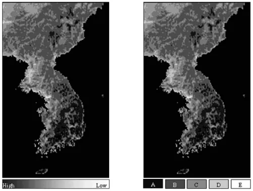
models of the whole area analyzed, which has four seasons. The constant mean level, amplitude and phase indices were estimated for this period using Eqs. (3), (4) and (5). Figs. 1, 2 and 3 shows the images of the estimated values of the harmonic components. The multi-temporal images of estimated NDVI for each component first were classified separately using the multistage algorithm.

The algorithm can use the values of the mean and amplitude indices directly for the similarity coefficient of Eq. (8), but the phase index must be transformed to an appropriate measure for the algorithm based on the difference of the values that represent the class. The phase index is a radian value with the range of ^_pand p.

The sine curve in the harmonic model of (1) is coincident at the two extreme values of phase, and the difference in this characteristic between classes is then not measured properly by the absolute difference of two phase indices. For example, the class with q = 5p/6 has more similar feature with the class with q = ^_5p/6 than the class with q = 0. A transformation was employed to overcome this problem, where the phase index is projected on the vector space of two dimensions:

v(q) =

[ ]

For the trigonometric component of Eq. (10), the value of one point in a quadrant is same as the value of another point that is located in one of the other quadrants, that is,

sinq = sin(p^_q) and cosq = cos(^_q),

whereas the values of two components are not same simultaneously at the same point. The distance measure based on this vector can properly quantify the difference in the phase index of class. However, if the merging in the clustering algorithm generates a new value of v(q) by combining two vectors of the merged sub-regions, the estimation may result in different values of phase index for each component. The merging algorithm must operate so that the estimate of the phase index after joining two groups is same in the two components. For

sinq cosq

Fig. 1. Image of estimated values (left) and classification image map (right) of mean index.

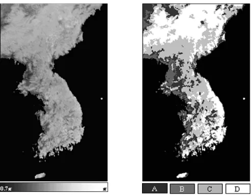
Fig. 2. Image of estimated values (left) and classification image map (right) of amplitude index.

this, the mean vector of Z = v(q) in Eq. (7) was estimated as follows:

m_j=

[ ]

where

q _

j= (sin^_1Sjsin

+ cos^_1Sjcos

), Sjsin

= sinqiand Sjcos

= cosqi.

Using identity matrix for the weight matrix, the similarity coefficient of the clustering for phase index is then

l_u= n_rmm’_rmm_r+ n_smm’_smm_s^_n_umm’_umm_u^_2(mm’_rS_r+ mm’_sS_s^_mm’_rS_s) (11) where

S_j=

[ ]

The classification results of each component are shown in Figs. 1, 2 and 3, and Tables 1. The algorithm generated 5, 5 and 4 classes for the mean, amplitude and phase indices respectively. In the classification image maps of Figs. 1 and 2 for the mean and amplitude

S_j^sin S_j^cos

S S

i∈Gj

1 n_j

S

i∈GSj

1 nj

1 2

sinq _

j

cosq _

j

Fig. 3. Image of estimated values (left) and classification image map (right) of phase index.

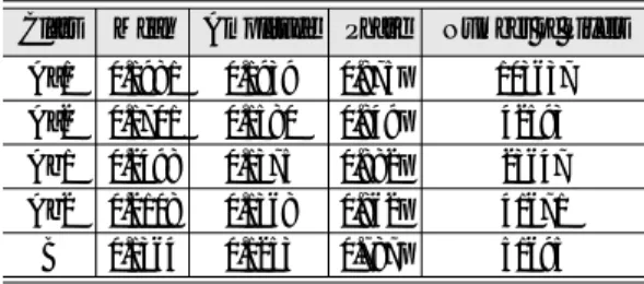
Table. 1. Estimated Values of Harmonic Components from Classification with Single Harmonic Component.

Class Mean Number of Pixels

A 0.2493 24270

B 0.2100 86832

C 0.1880 67159

D 0.1584 63861

E 0.1178 21121

Class Amplitude Number of Pixels

A 0.2147 24702

B 0.1897 80131

C 0.1631 57204

D 0.1385 58706

E 0.1011 42680

Class Phase Number of Pixels

A 0.750p 46253

B 0.813p 21799

C 0.858p 101407

D 0.889p 93784

Class Mean Number of Pixels

Class Amplitude Number of Pixels

Class Phase Number of Pixels

indices, the class with the higher class-average of each component is darker. As shown in Fig. 1, the annual- average values of NDVI are higher in the mountain region and the southern area of Korean Peninsula. Fig. 2 shows that the northern mountain area of the peninsula exhibits great seasonal variation in vegetation processes, but difference between the seasons is relatively small in the southern area. Fig. 3 displays the classification map of the phase index, in which the brighter shade represents the higher class-average, using Eq. (11). It shows that the highest peak of the yearly NDVI process generally comes earlier in the eastern area. Given the estimated phase index, qˆ, the highest point, t_p, can be obtained with monthly unit in a year:

_ qˆ, if qˆ<

tp= qˆshift× whereqˆ_shift= .

_ qˆ, otherwise

Next, the land cover of the Korean Peninsula was classified using the feature vector, which composes of three harmonic components estimated from the five year series of NDVI imagery. For this analysis, A and B in Eq. (2) were used instead of the amplitude and phase indices previously used because it is difficult to normalize the phase index in a same scale with the other components. Thus, the feature vector and the weight matrix for the distance measure of Eq. (7) are as follows:

Zi= and W =

where

sˆ²(z) =

is the estimated variance of z and the estimated mean intensity vector, mˆ_ziwas calculated with the average of the nine values of the center and eight nearest neighbor

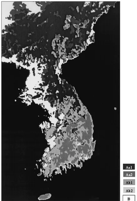
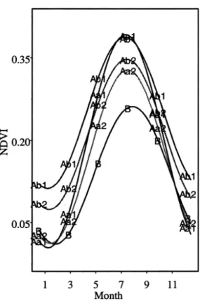
pixels in this study. The classification map is displayed in Fig. 4, and Table 2 and Fig. 5 contain the estimated harmonic function of observed NDVI for each class. As shown in Fig. 4, the land cover on the peninsula was classified with 5 classes. This classification is by and large summarized with northern vegetation area (Aa1, Aa2), southern vegetation area (Ab1, Ab2) and low vegetation area (B). Fig. 5 demonstrates that the level of NDVI is similar both in the north and south of the peninsula at the growing season, but it is much different at the low season. Classes Aa1 and Ab2 are closest in the estimated mean level, although the harmonic patterns of two classes are much different, as shown in

Table 2 and Fig. 5. It implies that the two classes are very possibly assigned in a same class, if the classification is performed with the similarity coefficient based only on the original values of NDVI observation.

5. Conclutions

Various multi-temporal techniques for analyzing remotely-sensed images have been developed, but conventional approaches for multi-temporal classification have usually used image data with low temporal resolution for a limited time period. An approach based on the harmonic model may be the most plausible temporal technique to analyze a sequence of the images that are acquired regularly at short time intervals for processes that exhibit seasonal trends such aˆ_i

Aˆi

Bˆ_i

3p 2 12

2p

p 2 p

2

Table. 2. Estimated Values of Harmonic Components from Classification with Three Harmonic Components.

Class Mean Amplitude Phase Number of Pixels Aa1 0.1981 0.1939 0.875p 103637 Aa2 0.1701 0.1580 0.849p 42593 Ab1 0.2498 0.1375 0.882p 23647 Ab2 0.2108 0.1368 0.862p 41671 B 0.1364 0.1253 0.787p 51695 Class Mean Amplitude Phase Number of Pixels

0 0

0 0

0 0 1

sˆ²(a) 1

sˆ²(a) 1

sˆ²(a)

(z_i^_mˆ_zi)’(z_i^_mˆ_zi) n

S

i∈ISn

as vegetation activity. However, spectral analysis is complicated when frequencies are unknown, thereby making this approach unsuitable for analyzing multi- temporal process observed in remote sensing data, where enormous amounts of data are usually examined.

Fortunately, most of vegetation processes assume one year cyclic behavior. Many studies have shown that the major agent of variability in NDVI data is inter-seasonal

phonological variability. The results of this study are consistent with this observation. For the NDVI processes, three temporal indices have been formulated from the harmonic model using the predetermined frequency. The mean index of the harmonic model represents the overall mean level of vegetation activity measured by NDVI, the amplitude and phase indices characterize the shape of the seasonal spectral profile.

Fig. 4. Classification image map using harmonic components.

These indices offer an alternative approach to the conventional techniques to discriminate between land- cover types based on the spectral signatures at a single or several points in time. To the extent that different vegetations have different development cycles, each type has a unique temporal profile. Thus, the classification reflects different sources of temporal variation by using the estimates that are obtained from sequential images through spectral analysis.

Ackknowledgement

This work was supported in part by the Kyungwon University and the Korean Ministry of Science and Technology (Grant #M60011000005- 02A0100-00410 ).

Reference

Zenzo, S. L., R. Bernstein, S. D. Degloria, and H. G.

Kolsky, 1987. Gaussian maximum likelihood and contextual classification algorithms for multicrop classification, IEEE Trans. Geosci.

Remote Sens., 25: 805-814.

Mohn, E., N. L. Hjort and G. O. Storvik, 1987.

Simulation study of some contextual classification methods for remotely sensed data, IEEE Trans. Geosci. Remote Sens., 25: 797-804.

Tucker, C. J., N. B. Hoblen, J. H. Elgin, Jr, and J. E.

Mcmurtey III, 1990. Relationship of spectral data to grain yield variation, Photogramm. Eng.

Remote Sens., 46: 657-666.

Teng, W. L., 1990. AVHRR monitoring of US. Crops during the 1988 drought, Photogramm. Eng.

Remote Sens., 56: 1143-1146.

Carlotto, M. J., 1985. Techniques for multispectral image classification, SPIE Digital Image Processing, 528: 174-191.

Goldberg, M., G. Karem, and M. Alvo, 1983. A production rule-based expert system for interpreting multi-temporal LANDSAT imagery, CVPR’83 Proceedings.

Horvath, N. C., T. I. Grey, and D. G. McCray, 1982.

Advanced Very High Resolution Radiometer (AVHRR) data evaluation for use in monitoring vegetation, AgRISTAR Report EW-L@-040303, JSC-18243, NASA, Lyndon B. Johnson Space Center, Houston, TX., 1982.0-1365.

Townsend, J. R. G. and C. J. Tucker, 1984. Objective assessment of AVHRR data for land cover mapping, Int. J. Remote Sens., 5: 492-501.

Tarpley, J. D., S. R. Schneider, and R. L. Money, 1984.

Global vegetation indices from the NOAA-7 meteorological satellite, J. Climate Appl.

Meteorol., 23: 491-494.

Fig. 5. Estimated harmonic functions for 5 classes.

Sampson, S. A., 1993. Two indices to characterize temporal patterns in the spectral response of vegetation, Photogramm. Eng. Remote Sens., 59: 511-517.

Lee, S-H, 2001. Unsupervised image classification using spatial region growing segmentation and hierarchical clustering, Korean Journal of Remote Sensing, 17: 57-70.

Bloomfield, P., 1976. Fourier Analysis of Time Series : An Introduction, John Wiley & Sons, Inc. New York.

Tanimoto, S. and A. Klinger, 1980. Structured Computer Vision, Academic, New York.

Anderberg, M. R., 1973. Cluster Analysis for Application, Academic Press, NewYork.

Holben, B. N., 1986. Characteristics of maximum value composite image from temporal AVHRR data, Int. J. Remote Sens., 7: 1417-1434.

Lee, S. and M. Crawford, 1991. Adaptive reconstruction system for spatially correlated multispectral multitemporal images, IEEE Trans. on Geosci.

Remote Sens., 29: 494-503.

Lee, S-H, 2002. Reconstruction and change analysis for temporal series of remotely-sensed data, Korean Journal of Remote Sensing, 18: 117-125.