1. Introduction
Formaldehyde (HCHO), one of most abundant aldehyde species, is produced from photo-oxidation of volatile organic compounds (VOCs). Moreover, HCHO plays an important role in the oxidation of VOCs, most of which are converted eventually to HCHO (Vrekoussis et al., 2010), which is then released
from biogenic, anthropogenic, and pyrogenic sources (De Smedt et al., 2010). Background levels of HCHO are generally determined by the amount of CH4, which exists in the troposphere at uniform concentrations on account of its stability (Heikes et al., 2001; Singh et al., 2001; Shim et al., 2005). Approximately 1600 Tg of HCHO is produced each year from the oxidation of CH4globally (Stavrakou et al., 2009). In addition to
Estimation of HCHO Column Using a Multiple Regression Method with OMI and MODIS Data
Hyunkee Hong1)·Jiwon Yang2)·Hyeongwoo Kang3)·Daewon Kim2)·Hanlim Lee 4)†
Abstract: We have estimated the vertical column density (VCD) of formaldehyde (HCHO) on a global scale using a multiple linear regression method (MRM) with Ozone Monitoring Instrument (OMI) and Moderate-Resolution Imaging Spectroradiometer (MODIS) data. HCHO VCDs were estimated in regions of biogenic, pyrogenic, and anthropogenic emissions using independent variables, including NO2VCD, land surface temperature (LST), an enhanced vegetation index (EVI), and the mean fire radiative power (MFRP), which are strongly correlated with HCHO. To evaluate the HCHO estimates obtained using the MRM, we compared estimates of HCHO VCD data measured by OMI (HCHOOMI) with those estimated by multiple linear regression equations (MRE) (HCHOMRE).
Good MRM performances were found, having the average statistical values (R = 0.91, slope = 1.03, mean bias = -0.12 × 10¹⁵molecules cm-2, percent difference = 11.27%) between HCHOMREand HCHOOMIin our study regions where high HCHO levels are present. Our results demonstrate that the MRM can be a useful tool for estimating atmospheric HCHO levels.
Key Words: multiple regression, formaldehyde, HCHO column, OMI, MODIS, trace gas estimation Korean Journal of Remote Sensing, Vol.35, No.4, 2019, pp.503~516
https://doi.org/10.7780/kjrs.2019.35.4.2 ISSN 1225-6161 ( Print )
ISSN 2287-9307 (Online)
Article
Received July 4, 2019; Revised July 16, 2019; Accepted July 31, 2019; Published online August 13, 2019
1)Researcher, Environmental Satellite Center, National Institute of Environmental Research; Postdoctoral Researcher, Department of Spatial Information Engineering, Pukyong National University
2)PhD Student, Department of Spatial Information Engineering, Pukyong National University
3)Master Student, Department of Spatial Information Engineering, Pukyong National University
4)Associate Professor, Department of Spatial Information Engineering, Pukyong National University
†Corresponding Author: Hanlim Lee ([email protected])
This is an Open-Access article distributed under the terms of the Creative Commons Attribution Non-Commercial License (http://creativecommons.org/licenses/by-nc/3.0) which permits unrestricted non-commercial use, distribution, and reproduction in any medium, provided the original work is properly cited.
VOC formation pathways, HCHO is also directly released into the atmosphere from biomass burning (Lee et al., 1997; Holzinger et al., 1999; Yokelson et al., 1999), fossil fuel combustion (Anderson et al., 1996; Geiger et al., 2002), and vegetation (Seco et al., 2007). However, such primary emissions of HCHO account for less than 1% of the global total. The presence of HCHO induces changes in tropospheric ozone levels, and the compound also plays an important role as a sink of the hydroxyl radical (OH) (Chance et al., 2000; Marais et al., 2014). Moreover, Formaldehyde has adverse effects on health, causing headaches and respiratory diseases; HCHO is also a known carcinogen (Xu et al., 2007).
To date, several environmental satellite sensors, such as the Global Ozone Monitoring Experiment (GOME) sensor on board the European Remote Sensing-2 (ERS-2) satellite (e.g., Thomas et al., 1998; Chance et al., 2000; Wittrock et al., 2006), the SCanning Imaging Absorption SpectroMeter for Atmospheric CHartographY (SCIAMACHY) on board the Environ - ment Satellite (ENVISAT) (De Smedt et al., 2008), the Ozone Monitoring Instrument (OMI) on board the Aura satellite (Gonzalez Abad et al., 2015) and the Atmospheric Chemistry Experiment-Fourier Transform Spectrometer (ACE-FTS) on board Science Satellite (SCISAT-1) (Dufour et al., 2009), have been monitoring the spatiotemporal distribution of atmospheric HCHO and its emission at regional and global scales since the mid-1990s. In addition, many studies have examined the distribution and origin of atmospheric HCHO and its precursors using the data obtained by such sensors.
Abbot et al. (2003) compared HCHO vertical column densities (VCDs) obtained by the GOME sensor and VCDs simulated by the Goddard Earth Observing System-Chem Model (GEOS-Chem) over North America. Martin et al. (2004) validated HCHO values obtained by the GOME sensor in comparisons with data obtained by in situ measurements over the Southeastern United States. A similar investigation was
also carried out over Asia. Witte et al. (2010) reported on characteristics of the HCHO/NO2ratio in China using OMI observations. Diurnal variations in HCHO were revealed from Multi Axis-Differential Optical Absorption Spectroscopy (MAX-DOAS) measurements during the 2006 Pearl River Delta Regions Campaign (PRIDE-PRD2006) in China (Li et al., 2013). De Smedt et al. (2010) investigated temporal trends in the tropospheric HCHO column in Asia using SCIAMACHY data. Similar studies have also been conducted to understand long-term trends in HCHO distributions on a global scale (e.g., De Smedt et al., 2010; Vrekoussis et al., 2010). Several studies (e.g., Shim et al., 2005; Marais et al., 2014) have examined the concentration distributions of HCHO using satellite- based observation data. Moreover, efforts have been made to estimate HCHO concentrations and its emission utilizing chemical transport models, such as GEOS-Chem, Community Multi-scale Air Quality Model (CMAQ), the Model of Emissions of Gases and Aerosol from Nature (MEGAN).
The multiple linear regression method (MRM) is one of the statistical methods for estimating concentrations of trace gas and aerosols. The MRM was used with Moderate-Resolution Imaging Spectroradiometer (MODIS) aerosol optical thickness (AOT) data to estimate the concentration of particulate matter less than 2.5 μm in size (PM2.5) (Gupta et al., 2009). Kim et al. (2012) calculated surface concentrations of primary organic carbon and secondary organic carbon using the MRM with in situ measurement data, and Abdul-Wahab et al. (2005) used the MRM to estimate ozone concentrations. The MRM based on a simple least square fitting procedure generally provides reliable estimations, with the variance depending on the characteristics of the independent and dependent variable data used in in the multiple linear regression equation (MRE). Choi et al. (2015) estimated HCHO column in major cities over Asia using MRM with satellite data. However, to date, no study has attempted
to estimate HCHO levels using the MRM on a global scale.
In this present study, we have, for the first time, estimated the HCHO VCD on a global scale using the MRM with OMI and MODIS data obtained in regions with high HCHO levels. Our aim was also to assess the high reliability of MRE-derived HCHO results, by comparing HCHO column data estimated by MREs (HCHOMRE) with those measured by OMI (HCHOOMI).
2. Method and data
1) Selection of data and variables for MRM
The MRM was used to estimate the spatial distribution of HCHO VCD using MREs consisting of a dependent and multiple independent variables.Regression coefficients, which determine the nature of the relationship, can be solved by the least squares fitting method (Timm, 2002). In the present study, HCHO VCD was the dependent variable. Since HCHO originates from primary sources and secondary formation related to biogenic, pyrogenic and anthropogenic sources, we selected independent variable candidates that represent each source type. Factors that are known to influence biogenic HCHO emissions include the leaf area index (LAI), land surface temperature (LST), leaf age, and photosynthetic active radiation (PAR) (Geron et al., 2000; Palmer et al., 2006). The LST influences the growth rates and productivity of plants, while the EVI reflects canopy cover, land cover, and the LAI (Liu et al., 1995; Gao et al., 1996; Matsushita et al., 2007).
Therefore, in this present study, the enhanced vegetation index (EVI) and LST were selected as the independent variable candidates influencing biogenic HCHO levels. LAI, however, is eventually excluded from the independent variable candidates due to its high value of variation inflation factor (VIF) against EVI.
The mean fire radiative power (MFRP) and NO2VCD
was selected as the independent variable candidates influencing pyrogenic HCHO levels. According to Barkley et al. (2009), biomass burning is a significant source of HCHO which implies that the stronger biomass burning can lead to the more HCHO produced.
Thus MFRP was selected independent variable candidate to reflect HCHO in biomass burning areas. NO2was also selected because biomass burning is a major source of NO2 (Andreae and Merlet, 2001). NO2was also selected as the independent variable candidate influencing anthropogenic HCHO levels since NO2is a known trace gas closely related to fossil fuel combustion and population density (Lamsal et al., 2013). High levels of nitrogen oxides (NOx) can lead to active oxidation of isoprene which is one of the precursor of the HCHO in physicochemical point of view (Trainer et al., 1987).
Furthermore, the accuracy of OMI NO2have relatively reliable even for the poor measurement conditions (e.g., high solar zenith angle and viewing zenith angle) since it uses visible wavelengths intensity is stronger than UV wavelengths, so that the MRM method may be helpful to compensate the operational OMI HCHO retrievals.
Although CO and CO2levels are also related to fossil fuel combustion, they were not used in the study on account of the large discrepancy between their lifetimes and that of HCHO.
The OMI and MODIS data were used as sources of data for the independent and dependent variables in the MRE. HCHO VCD, which is the dependent variable, is obtained from OMI observations (HCHOOMI) for the period from January 2005 to December 2008; the dates after December 2008 were constrained on account of a degradation problem with the OMI charge-coupled device (CCD) (http://disc.sci.gsfc.nasa.gov/Aura/data- holdings/OMI/index.shtml#info). Data for the other independent variables were also obtained for the same period as that of the HCHOOMIdata. The HCHOOMI
data were obtained from the OMI Formaldehyde Level2G Global binned data (OMHCHOG, v003). The HCHOOMIused in this present study are those with
cloud free (cloud fraction < 0.3) and those flagged as
“0” which means good quality level. NO2VCDs were obtained from the OMI Level-3 Global Gridded Total and Tropospheric NO2VCD Data Product (NO2OMI) (OMNO2d). The MODIS instrument on board the Terra and Aqua satellites, launched in 2000 and 2002, respectively, was in operation throughout the study period, providing daily products including LST, EVI, MFRP, etc. (Justice et al., 2002). The LST was obtained from the MODIS LST (LSTMODIS) dataset (MOD11C3) and the EVI was obtained from the MODIS EVI (EVIMODIS) dataset (MOD13C2). The MFRP was obtained from the MODIS MFRP (MFRPMODIS) dataset (MYD14CHM).
In this study, two criteria were applied in the selection of areas for estimating the HCHO VCD using the MRM; a) an absolute correlation coefficient (|R|) between HCHOOMIand at least two of the independent variable candidates greater than 0.4; b) a monthly maximum value of HCHOOMIwithin the top 30% of the global monthly average (i.e., > 2 × 10¹⁶molecules cm-2), as these areas are high in HCHO and are likely to show seasonal HCHO cycles.
The pyrogenic regions, where biomass burning is a dominant source of HCHO, and where correlations between HCHOOMIand both NO2OMIand MFRPMODIS
are high, include the Amazon (Barkley et al., 2008), South Borneo Island, Indochina Peninsula, and Southern Mexico. The regions, where oxidation of VOCs (such as isoprene) provides the dominant source of HCHO, include the Southeast United States, the correlation between HCHOOMIand both LSTMODISand EVIMODISis high, whereas no significant correlation is observed between HCHOOMIand MFRPMODIS. The regions, where high anthropogenic emissions of HCHO associated with fossil fuel combustion and population density is high, include Beijing, Nanjing, Seoul, NIIT, and New York. In areas of high anthropogenic emissions, annual mean NO2OMIlevels are greater than 1 × 10¹⁶molecules cm-2and high negative correlations are observed between
HCHOOMI and NO2OMI; however, no correlation is observed between HCHOOMIand MFRPMODISin these areas.
2) Study areas
To classify the regions into biogenic, pyrogenic, and anthropogenic source types, we investigated global
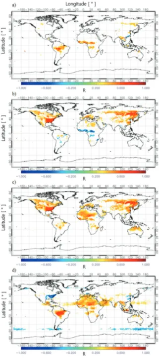
Fig. 1. Global distribution of the correlation coefficients (R) of linear regressions between HCHOOMI and (a) MFRPMODIS, (b) EVIMODIS, (c) LSTMODIS, and (d) NO2OMI, from 2005 to 2008.
distributions of the correlation coefficient (R) obtained from linear regressions between monthly means of HCHOOMIand MFRPMODIS, EVIMODIS, LSTMODIS, and NO2OMI, from 2005 to 2008 (Fig. 1(a)-(d), respectively).
Correlation coefficients in regions where satellite data are missing, or where data were observed at large solar zenith angles (SZAs), were excluded from Fig. 1. The negative correlations observed in high-latitude (~60°) regions can be attributed to large uncertainties in HCHOOMI and NO2OMI values related to the large SZA (Fig. 1(d)). Fig. 1(a) shows positive correlations between HCHOOMIand MFRPMODISin high-biomass regions (0.4-0.8), such as the Amazon [20°S-0°N, 50°W-70°W], Indochina [12°N-17°N, 100°E-108°E], and south Borneo Island [15°S-3°N, 110°E-120°E].
Fig. 1(b) shows negative correlations between HCHOOMI
and EVIMODIS(R = -0.6) in Africa and the Amazon, where biomass burning is a dominant source of HCHO. The average correlation between HCHOOMI
and EVIMODISin most temperate forests and grasslands in the Southeast United States [30°N-42°N, 80°W- 100°W] and East Asia [25°N-42°N, 112°E-140°E] is
~0.65. The spatial distribution of correlations between HCHOOMIand LSTMODISvalues (Fig. 1(c)) is similar to that between HCHOOMIand EVIMODIS(Fig. 1(b));
however, a positive correlation is observed in the Africa and Amazon regions (Fig. 1(c)). Fig. 1(d) shows that correlations between HCHOOMIand NO2OMIof -0.55 to -0.85 occur in the Southeastern United States, the industrialized area in the eastern coastal region of China, the Northern Italy Industrial Triangle (NIIT;
Turin, Milan, and Genoa), and in northeast Asian megacities, such as Beijing and Seoul.
3) Multiple regression method
The MRE can be defined as following equation:
Y = a0+ a1X1+ a2X2… + anXn+ ε (1) Here, Y is dependent variable (HCHOMRE), a0 is constant coefficient, X1, X2, …, Xnare the independent
variables (NO2 OMI, LSTMODIS, EVIMOIDS, and MFRPMODIS), a1, a2, …, an are the regression coefficient, and ε is the difference between observations (HCHOOMI) and estimated values (HCHOMRE). The regression coefficients can be estimated by the least square fitting (Equation 2).
∑mj=1εj2= ∑mj=1(yj–^yj)2 (2) Where yj is observed value with m numbers of data points. By minimizing the sum of ε2, regression coefficients can be derived. Among the four independent variable candidates described in Section 2.1, to select optimal independent variables used in the MREs, two criteria were applied: variation inflation factor (VIF) and p-value. First, we examined the VIF that quantifies the multicollinearity of an independent variable candidate with regard to other independent variable candidates.
The VIF of the j-th independent variable is expressed as:
1
VIF(xj) = ——– (3) 1 – Rj2
Where Rj2is the R-squared value for the regression of xjagainst the other covariates (a regression that does not involve the dependent variable j). The VIF indicates how much xj is correlated with the variables. A candidate for independent variable with a very high VIF can be considered redundant and should be removed from the MRE. The candidates for independent variables, which do not satisfy the criterion VIF > 10 (Kutner et al., 2004), were excluded from the independent variables. We also used p-value to select independent variables. The significance level is set to 0.05 (5%) (Sellke et al., 2001). Among the independent variable candidates that satisfy the VIF criterion, those that also satisfy the p-value less than 0.05 (p-value < 0.05) are selected as final independent variables in the MRE. The independent variables and regression coefficients determined by least square fitting for each area are shown in Table 1.
4) Monthly characteristics of the variables used in MRE
Temporal tendencies and amplitudes between the dependent variable (HCHOOMI) and the independent variable candidates (NO2OMI, LSTMODIS, EVIMODIS, and MFRPMODIS) are important for obtaining optimal regression coefficients for the MRE. To understand how temporal trends and amplitudes HCHOOMIand the other independent variable candidates depend on biogenic, pyrogenic, and anthropogenic source areas,
we investigated the temporal characteristics of HCHOOMI
and the other independent variable candidates that are strongly correlated with HCHOOMIin different geographic areas (see Fig. 2, 3 and 4).
(1) Biomass burning (pyrogenic) regions
Fig. 2 shows the time series of HCHOOMI, LSTMODIS, NO2OMI, and MFRPMODIS from 2005 to 2008 in the pyrogenic regions: (a) Amazon, (b) south Borneo, (c) south Mexico, and (d) Indochina. In general, the temporal cycles and amplitudes of the variables are in
Fig. 2. Time series of HCHOOMI, LSTMODIS, NO2OMI, and MFRPMODIS(see text for an explanation of these variables) in different pyrogenic source regions of HCHO: (a) Amazon, (b) south Borneo, (c) south Mexico, (d) Indochina.
good agreement, which implies, for example, that both HCHOOMI and NO2OMI are emitted from periodic biomass burning events in savanna and tropical forests, as has also been reported in previous studies (Barkley et al., 2008; Marais et al., 2012). Monthly average MFRPMODISvalues in the Amazon in September 2008 were 30% lower than those in 2005 and 2006 (Fig. 2(a)).
Similarly, monthly averages of HCHOOMI(2.7 × 10¹⁶ molecules cm-2) and NO2OMI (5.0 × 10¹⁵molecules cm-2) in September 2008 were 80% of those in 2005 and 70% of those in 2006, respectively. The MFRPMODIS
values observed during the biomass burning period from July to October in south Borneo were 30%
higher in 2006 than in 2005, 2007, and 2008 (Fig. 2(b)).
During the biomass burning period in 2006, monthly average of HCHOOMIwas 4.0 × 10¹⁶molecules cm-2; this value is also approximately 60% higher than those in 2005, 2007, and 2008. Monthly average of NO2OMIwas 5.7 × 10¹⁵molecules cm-2; this value is also approximately 45% higher than those in 2005, 2007, and 2008. Temporal characteristics of HCHOOMIin central Africa were different from those in other pyrogenic regions. In central Africa, seasonal cycles of NO2OMIand MFRPMODISwere similar to those in other pyrogenic areas; however, the trend of decreased HCHOOMIin January corresponding to maximum levels of MFRPMODISis unique to this region. The causes of this unique trend in HCHOOMIlevels in January have not been so far examined, and this subject requires further investigations.
(2) Biogenic regions
Fig. 3 shows time series of HCHOOMI, NO2OMI, EVIMODIS, and LSTMODIS in biogenic regions: the Southeastern United States. Levels of HCHOOMI, LSTMODIS, and EVIMODIStend to increase in summer and are strongly correlated with one another. In the southeast United States, HCHO levels are reported to originate from biogenic sources, such as deciduous forests, woodland regeneration, CH4oxidation, and industrial emissions (Shim et al., 2005; Millet et al., 2008). Annual cycles of HCHOOMIare similar to those of both LSTMODIS and EVIMODIS, which implies that biogenic sources are dominant in this area.
(3) Anthropogenic regions
Fig. 4 shows time series of HCHOOMI, NO2OMI, EVIMODIS, and LSTMODISin anthropogenic regions: Seoul, Beijing, Nanjing, Atlanta, New York, and NIIT. Fig. 5 shows correlations between HCHOOMI and NO2OMI in the representative anthropogenic areas of Seoul, New York, and NIIT from 2005 to 2008. Levels of HCHOOMIare strongly correlated with EVIMODISand LSTMODISin the representative anthropogenic areas, as shown in Fig. 4.
The similarity of temporal cycles of EVIMODIS and LSTMODIScan be attributed to the locations in temperate climate regions in the Northern Hemisphere. However, the similarity of seasonal cycles of HCHOOMIwith those of EVIMODIS does not necessarily mean that HCHO is affected by EVI, but that the two are both related to increased secondary formation of HCHO
Fig. 3. Time series of HCHOOMI, NO2OMI, EVIMODIS, and LSTMODIS(see text for an explanation of these variables) in biogenic source regions of HCHO: southeast United States.
Fig. 4. Time series of HCHOOMI, LSTMODIS, EVIMODIS, and NO2OMI(see text for an explanation of these variables) in different anthropogenic source regions of HCHO: (a) Seoul, (b) Beijing, (c) Nanjing, (d) Atlanta, (e) New York, and (f) NIIT.
from anthropogenic VOCs under conditions of enhanced solar radiation. The negative correlation between HCHOOMIand NO2OMIin biogenic areas is much smaller than that in anthropogenic areas. The correlation between HCHOOMIand NO2OMIis -0.66 in the southeast United States, and is -0.53 and -0.37 in biogenic regions such as the states of Alabama and Georgia, respectively. However, high negative correlations between HCHOOMIand NO2OMIoccur in anthropogenic areas in North America such as New York and Atlanta (-0.77 and -0.84, respectively). Similarly, strong negative correlations between HCHOOMIand NO2OMIoccur in Seoul and NIIT (-0.76 and -0.79, respectively) (Fig. 5).
Levels of HCHOOMIand NO2OMIare strongly correlated in anthropogenic areas, as HCHO and NO2exhibit both opposite seasonal cycles and also large-amplitude variations.
3. Results 1) Determination of the MREs
Monthly average values of NO2OMI, LSTMODIS, EVIMODIS, and MFRPMODISwere used as the independent variable candidates in the MRE, and that of HCHOOMI
was used as the only dependent variable. All monthly datasets from 2005 through 2008 (N = 48), which were used to determine MREs. Regression coefficients were determined using a linear least squares fitting method (Timm, 2002). The NO2OMIvariable was categorized into two types depending on the dominant NO2source type in each area: NO2_BBwas used to represent the NO2 in pyrogenic-dominant regions, such as the Amazon, south Borneo, south Mexico, and Indochina, whereas NO2_FFwas used to represent the NO2in anthropogenic- Fig. 5. Correlation between HCHOOMIand HCHONO2at (a) Seoul, (b) New York, and (c) NIIT between January 2005
and December 2008. Black lines are regression lines calculated using two measurement datasets.
dominant areas (Fossil fuel), such as Seoul, Beijing, Nanjing, New York, Atlanta, and NIIT. The best least squares fit was achieved in the pyrogenic areas when
NO2_BB, LSTMODIS, MFRPMODIS, and EVIMODISwere used as the independent variables, as shown in Table 1.
Table 1 shows that R2values range from 0.62 to Table 1. Coefficients of the multiple regression equations (MRE) used to predict HCHO (HCHOMRE), and coefficient of
determination (R2) for the linear regressions between HCHOOMIand HCHOMRE, for different regions
Type Regions VIFa p-valueb Beta (β)
weight Multiple regression equationc R2d Pyrogenic-dominant
regions
Amazon South Borneo South Mexico Indochina
MFRP(0.81) (0.40)EVI
NO2_BB (0.717) (0.167)LST
3.74 × NO2_BB+ 0.32 × LST – 8.25 0.69 Biogenic-dominant
region Southeast United
States LST
(11.50) NO2
(0.21) EVI
(0.918) 36.55 × EVI – 0.14 0.84
Anthropogenic- dominant
Regions
Seoul Beijing Nanjing Atlanta New York
NIIT
NO2_FF (0.321) (0.441)LST (0.578)EVI
0.31 × NO2_FF+ 0.20 × LST + 20.26
× EVI – 0.78 0.62
Notes: NO2and HCHO are column densities (× 1015molecules cm-2).
aThe independent variable candidates that do not satisfy the VIF criterion (VIF < 10) are listed.
bThe independent variable candidates that do not satisfy p-value criterion (p-value < 0.05) are listed.
cMFRP is excluded from independent variable for MREs in Anthropogenic regions.
dCoefficient of determination between HCHOOMIand HCHOMRE.
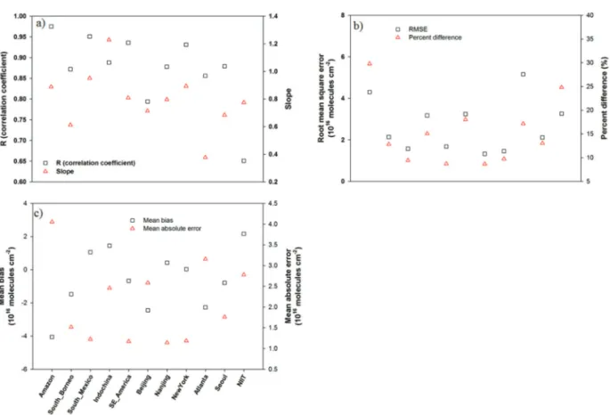
Fig. 6. Slopes and correlation coefficient (a), root mean square error (RMSE) and percent difference (b), and mean bias error and mean absolute error (c) obtained from the linear regressions between HCHOOMIand HCHOMRE.
0.84, indicating that HCHOMREis in good agreement with HCHOOMI. In pyrogenic-dominant regions such as Amazon, South Borneo, South Mexico, and Indochina, the best estimates of HCHO were obtained when NO2_BB, LSTMODISwere used as independent variables in the MRE; note that MFRPMODIS was excluded due to a high p-value from the final MREs in several pyrogenic regions (see Table 1). The R2 between HCHOMREand HCHOOMIrepresents 0.69. In biogenic- dominant regions, the southeast United States, the best HCHO estimate was achieved when EVIMODISwere used as independent variables (R2= 0.84) (see Table 1).
In anthropogenic-dominant regions, the best estimates of HCHO were obtained when NO2_FF, EVIMODIS, and LSTMODISwere used as independent variables in the MRE. The R2between HCHOMREand HCHOOMI
is 0.62.
Fig. 6(a) shows the slopes and correlation coefficient obtained from the linear regressions between HCHOOMI
and HCHOMRE. The correlation coefficient (R) and the slopes are found to be up to 0.97 and 0.94, respectively, showing very good agreements between HCHOOMIand HCHOMRE. Fig. 6(b) presents root mean square error (RMSE) and percent difference obtained from the linear regressions between HCHOOMIand HCHOMRE. The RMSE and percent difference are found to be up to 2.5 and 25%, respectively, showing good performances of MRM. The mean bias values are found to be either close to or slightly smaller than zero in Fig. 6(c), implying negligible bias of HCHOMRE against HCHOOMI.
4. Conclusions
To estimate HCHO levels in pyrogenic regions, such as the Amazon, south Borneo, south Mexico, and Indochina, the independent variables NO2_BB, LSTMODIS, and MFRPMODIS were used in MREs. In biogenic regions such as the Southeastern United States,
LSTMODIS, and EVIMODISwere used as the independent variables in the MRE. In anthropogenic regions, such as Seoul, Beijing, Nanjing, New York, Atlanta, and NIIT, NO2_FF, LSTMODIS, and EVIMODISwere used as the independent variables. The HCHOMREvalues were in good agreement with HCHOOMIvalues in most regions.
Acknowledgements
This work was supported by a Research Grant of Pukyong National University (2017 year).
References
Abbot, D. S., P. I. Palmer, R. V. Martin, K. V.
Chance, D. J. Jacob, and A. Guenther, 2003.
Seasonal and interannual variability of North American isoprene emissions as determined by formaldehyde column measurements from space, Geophysical Research Letters, 30(17).
Abdul-Wahab, S. A., C. S. Bakheit, and S. M.
Al-Alawi, 2005. Principal component and multiple regression analysis in modelling of ground-level ozone and factors affecting its concentrations, Environmental Modelling &
Software, 20(10): 1263-1271.
Anderson, L. G., J. A. Lanning, R. Barrell, J.
Miyagishima, R. H. Jones, and P. Wolfe, 1996. Sources and sinks of formaldehyde and acetaldehyde: An analysis of Denver’s ambient concentration data, Atmospheric Environment, 30(12): 2113-2123.
Andreae, M. O., and P. Merlet, 2001. Emission of trace gases and aerosols from biomass burning, Global Biogeochemical Cycles, 15(4): 955-966.
Barkley, M. P., P. I. Palmer, U. Kuhn, J. Kesselmeier, K. Chance, T. P. Kurosu, R. V. Martin, D.
Helmig, and A. Guenther, 2008. Net ecosystem fluxes of isoprene over tropical South America inferred from Global Ozone Monitoring Experiment (GOME) observations of HCHO columns, Journal of Geophysical Research:
Atmospheres, 113(D20).
Bey, I., D. J. Jacob, R. M. Yantosca, J. A. Logan, B. D.
Field, A. M. Fiore, Q. Li, H. Y. Liu, L. J.
Mickley, and M. G. Schultz, 2001. Global modeling of tropospheric chemistry with assimilated meteorology: Model description and evaluation, Journal of Geophysical Research:
Atmospheres, 106(D19): 23073-23095.
Boeke, N. L., J. D. Marshall, S. Alvarez, K. V. Chance, A. Fried, T. P. Kurosu, B. Rappengluck, D. Richter, J. Walega, and P. Weibring, 2011.
Formaldehyde columns from the Ozone Monitoring Instrument: Urban versus background levels and evaluation using aircraft data and a global model, Journal of Geophysical Research: Atmospheres, 116(D5).
Chance, K., P. I. Palmer, R. J. D. Spurr, R. V. Martin, T. P. Kurosu, and D. J. Jacob, 2000. Satellite observations of formaldehyde over North America from GOME, Geophysical Research Letters, 27(21): 3461-3464.
Choi, W., H. Hong, J. Park, and H. Lee, 2015. First- time estimation of HCHO column in major cities over Asia using multiple regression with satellite data, Korean Journal of Remote Sensing, 31(6): 523-530 (in Korean with English abstract).
De Smedt, I., J. F. Müller, T. Stavrakou, R. Van Der A, H. Eskes, and M. Van Roozendael, 2008.
Twelve years of global observations of formaldehyde in the troposphere using GOME and SCIAMACHY sensors, Atmospheric Chemistry and Physics, 8: 4947-4963.
De Smedt, I., T. Stavrakou, J. F. Muller, R. Van Der A, and M. Van Roozendael, 2010. Trend detection
in satellite observations of formaldehyde tropospheric columns, Geophysical Research Letters, 37(18).
Dufour, G., S. Szopa, M. P. Barkley, C. D. Boone, A. Perrin, P. I. Palmer, and P. F. Bernath, 2009. Global upper-tropospheric formaldehyde:
seasonal cycles observed by the ACE-FTS satellite instrument, Atmospheric Chemistry and Physics, 9(12): 3893-3910.
Fu, T. M., D. J. Jacob, P. I. Palmer, K. Chance, Y. X. Wang, B. Barletta, D. R. Blake, J. C.
Stanton, and M. J. Pilling, 2007. Space-based formaldehyde measurements as constraints on volatile organic compound emissions in east and south Asia and implications for ozone, Journal of Geophysical Research:
Atmospheres, 112(D6).
Geiger, H., J. Kleffmann, and P. Wiesen, 2002. Smog chamber studies on the influence of diesel exhaust on photosmog formation, Atmospheric Environment, 36(11): 1737-1747.
Geron, C., A. Guenther, T. Sharkey, and R. R. Arnts, 2000. Temporal variability in basal isoprene emission factor, Tree Physiology, 20(12): 799- 805.
Gonzalez Abad, G., X. Liu, K. Chance, H. Wang, T. P.
Kurosu, and R. Suleiman, 2015. Updated Smithsonian Astrophysical Observatory Ozone Monitoring Instrument (SAO OMI) formaldehyde retrieval, Atmospheric Measurement Techniques, 8(1): 19-32.
Gupta, P. and S. A. Christopher, 2009. Particulate matter air quality assessment using integrated surface, satellite and meteorological products:
Multiple regression approach, Journal of Geophysical Research: Atmospheres, 114(D14).
Heikes, B., J. Snow, P. Egli, D. O’Sullivan, J. Crawford, J. Olson, G. Chen, D. Davis, N. Blake, and D.
Blake, 2001. Formaldehyde over the central Pacific during PEM-Tropics B, Journal of
Geophysical Research: Atmospheres, 106(D23):
32717-32731.
Holzinger, R., C. Warneke, A. Hansel, A. Jordan, W.
Lindinger, D. H. Scharffe, G. Schade, and P. J.
Crutzen, 1999. Biomass burning as a source of formaldehyde, acetaldehyde, methanol, acetone, acetonitrile, and hydrogen cyanide, Geophysical Research Letters, 26(8): 1161- 1164.
Jeong, J. I. and R. J. Park, 2013. Effects of the meteorological variability on regional air quality in East Asia, Atmospheric Environment, 69:
46-55.
Justice, C., J. Townshend, E. Vermote, E. Masuoka, R.
Wolfe, N. Saleous, D. Roy, and J. Morisette, 2002. An overview of MODIS Land data processing and product status, Remote Sensing of Environment, 83(1-2): 3-15.
Kim, W., H. Lee, J. Kim, U. Jeong, and J. Kweon, 2012. Estimation of seasonal diurnal variations in primary and secondary organic carbon concentrations in the urban atmosphere: EC tracer and multiple regression approaches, Atmospheric Environment, 56: 101-108.
Lee, M., B. G. Heikes, D. J. Jacob, G. Sachse, and B.
Anderson, 1997. Hydrogen peroxide, organic hydroperoxide, and formaldehyde as primary pollutants from biomass burning, Journal of Geophysical Research: Atmospheres, 102(D1):
1301-1309.
Li, X., T. Brauers, A. Hofzumahaus, K. Lu, Y. Li, M.
Shao, T. Wagner, and A. Wahner, 2013. MAX- DOAS measurements of NO2, HCHO and CHOCHO at a rural site in Southern China, Atmospheric Chemistry and Physics, 13(4):
2133-2151.
Marais, E. A., D. J. Jacob, T. Kurosu, K. Chance, J.
Murphy, C. Reeves, G. Mills, S. Casadio, D.
Millet, and M. P. Barkley, 2012. Isoprene emissions in Africa inferred from OMI
observations of formaldehyde columns, Atmospheric Chemistry and Physics, 12(14):
6219-6235.
Marais, E. A., D. Jacob, A. Guenther, K. Chance, T.
Kurosu, J. Murphy, C. Reeves, and H. Pye, 2014. Improved model of isoprene emissions in Africa using OMI satellite observations of formaldehyde: implications for oxidants and particulate matter, Atmospheric Chemistry and Physics Discussions, 14(5): 6951-6979.
Martin, R., D. Parrish, T. Ryerson, D. Nicks, K.
Chance, T. Kurosu, D. Jacob, E. Sturges, A.
Fried, and B. Wert, 2004. Evaluation of GOME satellite measurements of tropospheric NO2
and HCHO using regional data from aircraft campaigns in the southeastern United States, Journal of Geophysical Research: Atmospheres, 109(D24).
Matsushita, B., W. Yang, J. Chen, Y. Onda, and G. Qiu, 2007. Sensitivity of the enhanced vegetation index (EVI) and normalized difference vegetation index (NDVI) to topographic effects:
a case study in high-density cypress forest, Sensors, 7(11): 2636-2651.
Michael H. K., C. J. Nachtsheim, J. Neter, and W. Li, 2005. Applied Linear Regression Models (Vol.
5), McGraw-Hill/Irwin, New York, NY, USA.
Lamsal, L., R. Martin, D. D. Parrish, and N. A. Krotkov, 2013. Scaling relationship for NO2pollution and urban population size: A satellite perspective, Environmental Science & Technology, 47(14):
7855-7861.
Millet, D. B., D. J. Jacob, K. F. Boersma, T. M. Fu, T.
P. Kurosu, K. Chance, C. L. Heald, and A.
Guenther, 2008. Spatial distribution of isoprene emissions from North America derived from formaldehyde column measurements by the OMI satellite sensor, Journal of Geophysical Research: Atmospheres, 113(D2).
Palmer, P. I., D. S. Abbot, T. M. Fu, D. J. Jacob, K.
Chance, T. P. Kurosu, A. Guenther, C.
Wiedinmyer, J. C. Stanton, and M. J. Pilling, 2006. Quantifying the seasonal and interannual variability of North American isoprene emissions using satellite observations of the formaldehyde column, Journal of Geophysical Research: Atmospheres, 111(D12).
Park, R. J., D. J. Jacob, B. D. Field, R. M. Yantosca, and M. Chin, 2004. Natural and transboundary pollution influences on sulfate-nitrate-ammonium aerosols in the United States: Implications for policy, Journal of Geophysical Research:
Atmospheres, 109(D15).
Qing Liu, H. and A. Huete, 1995. A feedback based modification of the NDVI to minimize canopy background and atmospheric noise, IEEE Transactions on Geoscience and Remote Sensing, 33(2): 457-465.
Seco, R., J. Penuelas, and I. Filella, 2007. Short-chain oxygenated VOCs: Emission and uptake by plants and atmospheric sources, sinks and concentrations, Atmospheric Environment, 41(12): 2477-2499.
Sellke, T., M. J. Bayarri, and J. O. Berger, 2001.
Calibration of ρ values for testing precise null hypotheses, The American Statistician, 55(1):
62-71.
Shim, C., Y. Wang, Y. Choi, P. I. Palmer, D. S. Abbot, and K. Chance, 2005. Constraining global isoprene emissions with Global Ozone Monitoring Experiment (GOME) formaldehyde column measurements, Journal of Geophysical Research:
Atmospheres, 110(D24).
Singh, H., L. Salas, R. Chatfield, E. Czech, A. Fried, J.
Walega, M. Evans, B. Field, D. Jacob, and D.
Blake, 2004. Analysis of the atmospheric distribution, sources, and sinks of oxygenated
volatile organic chemicals based on measurements over the Pacific during TRACE-P, Journal of Geophysical Research: Atmospheres, 109(D15).
Stavrakou, T., J.-F. Muller, I. D. Smedt, M. V.
Roozendael, G. van der Werf, L. Giglio, and A.
Guenther, 2009. Evaluating the performance of pyrogenic and biogenic emission inventories against one decade of space-based formaldehyde columns, Atmospheric Chemistry and Physics, 9(3): 1037-1060.
Timm, N. H., 2002. Applied Multivariate Analysis:
Springer Texts in Statistics, Springer-Verlag New York, NY, USA.
Vrekoussis, M., F. Wittrock, A. Richter, and J. Burrows, 2010. GOME-2 observations of oxygenated VOCs: what can we learn from the ratio glyoxal to formaldehyde on a global scale?, Atmospheric Chemistry and Physics, 10(21):
10145-10160.
Witte, J. C., B. N. Duncan, A. R. Douglass, T. P.
Kurosu, K. Chance, and C. Retscher, 2011.
The unique OMI HCHO/NO2feature during the 2008 Beijing Olympics: Implications for ozone production sensitivity, Atmospheric Environment, 45(18): 3103-3111.
Xu, J., X. Jia, X. Lou, G. Xi, J. Han, and Q. Gao, 2007. Selective detection of HCHO gas using mixed oxides of ZnO/ZnSnO3, Sensors and Actuators B: Chemical, 120(2): 694-699.
Yokelson, R. J., J. G. Goode, D. E. Ward, R. A. Susott, R. E. Babbitt, D. D. Wade, I. Bertschi, D. W.
Griffith, and W. M. Hao, 1999. Emissions of formaldehyde, acetic acid, methanol, and other trace gases from biomass fires in North Carolina measured by airborne Fourier transform infrared spectroscopy, Journal of Geophysical Research: Atmospheres, 104(D23): 30109-30125.