다중 표준 유전체 분석을 통한 고추 속 식물의 유전체 진화 및 종 분화 연구

(1)

저작자표시-비영리-변경금지 2.0 대한민국 이용자는 아래의 조건을 따르는 경우에 한하여 자유롭게 l 이 저작물을 복제, 배포, 전송, 전시, 공연 및 방송할 수 있습니다. 다음과 같은 조건을 따라야 합니다: l 귀하는, 이 저작물의 재이용이나 배포의 경우, 이 저작물에 적용된 이용허락조건 을 명확하게 나타내어야 합니다. l 저작권자로부터 별도의 허가를 받으면 이러한 조건들은 적용되지 않습니다. 저작권법에 따른 이용자의 권리는 위의 내용에 의하여 영향을 받지 않습니다. 이것은 이용허락규약(Legal Code)을 이해하기 쉽게 요약한 것입니다. Disclaimer 저작자표시. 귀하는 원저작자를 표시하여야 합니다. 비영리. 귀하는 이 저작물을 영리 목적으로 이용할 수 없습니다. 변경금지. 귀하는 이 저작물을 개작, 변형 또는 가공할 수 없습니다.

(2)

A DISSERTATION FOR THE DEGREE OF DOCTOR OF PHILOSOPHY

Multiple Reference Pepper Genome

Analysis Provides Insights into Genome

Evolution and Speciation of Capsicum spp.

다중 표준 유전체 분석을 통한 고추 속 식물의

유전체 진화 및 종 분화 연구

AUGUST 2015

SEUNGILL KIM

INTERDISCIPLINARY PROGRAM IN AGRICULTURAL BIOTECHNOLOGY COLLEGE OF AGRICULTURE AND LIFE SCIENCES

(3)

(4)

i

Multiple Reference Pepper Genome Analysis Provides

Insights into Genome Evolution and Speciation of

Capsicum spp.

SEUNGILL KIM

Interdisciplinary Program in Agricultural Biotechnology,

Seoul National University

ABSTRACT

Pepper (Capsicum spp.) is widely cultivated spice crop and a major ingredient of worldwide cuisines. In this study, a high-quality reference genome of hot pepper (Capsicum annuum CM334) was constructed containing genome assembly, annotation and chromosome pseudomolecules. A total of 87.9 % (3.06 Gb) of 3.48 Gb genome was assembled and 2.63 Gb of the assembled sequence was integrated into twelve chromosomes. By comparing to the completed BAC sequences, the assembled genome was validated and the validation result showed that the identities between the assembled genome and BAC sequences were more than 99%. A total of 34,903 protein-coding genes were predicted and their biological functions were annotated. To

(5)

ii

construct multiple reference genomes of the genus Capsicum, high-quality de novo genome sequences of two domesticated Capsicum spp. (C. chinense and C. baccatum) were obtained and comparative analysis with C. annuum CM334 genome was performed. The phylogenetic analysis revealed that the speciation of the Capsicum species has occurred at approximately between one and two million years ago. The genome size variation between C. baccatum and the other Capsicum spp. was caused by excessive accumulation of athila subgroup of LTR/Gypsy retrotransposon. The insertion pattern of LTR-retrotransposons was represented that the accumulation of LTRs for C. chinense and C. baccatum were distinctly increased around their speciation time. Comparative and evolutionary analysis of gene families unveiled that the expanded gene families in each pepper genome were actively increased by recent gene duplication event occurred around the speciation times. The high-quality multiple reference genomes of the genus Capsicum will provide a versatile platform for genetic and genomic improvements as well as essential resources to promote population and comparative genomic studies in the genus Capsicum.

Keywords: genome, Capsicum annuum, Capsicum baccatum, Capsicum chinense, next generation sequencing (NGS), assembly, annotation, speciation, genome evolution, transposable elements (TEs), LTR-retrotransposons, compartive genomic analysis

(6)

iii

LIST OF TABLES

CHAPTER 1

Table 1. Hot pepper genome sequence generated in this study ……….…19 Table 2. Details of CM334 genome assembly ….……...……….…24 Table 3. Statistics of CM334 genome assembly ………..25 Table 4. Summary of validation of the CM334 genome assembly using 27 BAC clones ………..27 Table 5. Summary of linkage groups from subdivided markers groups ………...32 Table 6. Summary of the integrated 12 linkage groups ……….…33 Table 7. Details of the 12 chromosome pseudomolecules..……….…36 Table 8. Validation of pseudomolecules using COS markers……….…37 Table 9. Classification summary of transposable elements (TEs) of pepper genome………39 Table 10. Properties of transcriptome used for gene annotation……….……….…43 Table 11. Training set for ab initio gene prediction……….…44 Table 12. Metrics of pepper gene models……….…46

CHAPTER 2

(10)

vii

Table 2. Generated C. baccatum genome sequences in this study …..………70 Table 3. Comparison of the pepper genome assemblies ……….……..72 Table 4. Statistics of twelve pseudomolecule chromosomes of the pepper genomes.75 Table 5. Comparison of annotated gene models of the pepper genomes….……….76 Table 6. Protein sets used for gene family analysis……….…77 Table 7. Number of expanded gene families in the three pepper genomes……..…82 Table 8. Amount of repeat sequences in whole genome of the peppers.……….…87 Table 9. Amount of Gypsy subgroups in the pepper genomes……….…89 Table 10. Total volume of Copia subgroups in the pepper genomes……….90 Table 11. Statistics of Caulimoviridae subgroups in the pepper genomes……….91

(11)

viii

LIST OF FIGURES

CHAPTER 1

Fig. 1. The 19-mer depth distribution for the raw sequence data of pepper genome..21 Fig. 2. Distribution of insert size for pepper genome……….……….22 Fig. 3. Detailed visualization of validation of CM334 genome assembly against 27 BAC sequences………..……..28 Fig. 4. Genetic and physical maps of CM334 genome……..……….……….35 Fig. 5. Global overview of the pepper genome……….………….………..40 Fig. 6. Histogram of pairwise comparison of protein length ratios with their best blast hit relative to the reference pepper and tomato versus potato…..……….47 Fig. 7. The top 20 INTERPRO domains in PGA version.1.5……….……….49 Fig. 8. Scheme of raw data processing pipeline………….………….……….….51

CHAPTER 2

Fig. 1. Gene annotation scheme for the pepper genomes ..……….……...66 Fig. 2. The 19-mer distribution of the sequenced pepper genomes ……….71 Fig. 3. Strategy for pseudomolecule construction of the C. baccatum and C. chinense………...73 Fig. 4. Comparison of the orthologous gene families….……..……….…….79 Fig. 5. Estimated divergence time of the sequenced plant genomes….….……….80 Fig. 6. Biological function of the expanded gene families in the pepper genomes….83

(12)

ix

Fig. 7. Age of the expanded gene families in the pepper genomes ...……….…….84 Fig. 8. FISH with 25S (red) ribosomal DNA probes to somatic metaphase chromosomes of Capsicum species………92 Fig. 9. Comparison for ratio of subgroups between intact and whole LTR

-retrotransposons………..……….………..………….94 Fig. 10. Age of LTR-retrotransposons in the pepper genomes………..95

(13)

x

LIST OF ABBREVIATIONS

NGS next generation sequencing WGS whole genome shotgun TEs transposable elements LTR long terminal repeat

BAC bacterial artificial chromosome FAO food and agriculture organization PE paired-end

MP mate-pair

RIL recombinant inbred line PGA pepper gene annotation EVM evidence modeler

COS conserved orthologue set OrthoMCL ortholog markov cluster

BEAST bayesian evolutionary analysis sampling trees MYA million years ago

(14)

1

GENERAL INTRODUCTION

Since the first plant genome sequencing project, Arabidopsis thaliana, was completed in 2000, a wide variety of plant genome sequences were reported including plants with different genome size ranging from 125Mb (Arabidopsis thaliana) to 20.0 Gb (Pinus taeda)1-3. Compared to other eukaryotic genomes, plant genomes are usually larger in size and highly enriched with repeat sequences. These features have been barriers of the genome assembly, and required enormous amount of sequencing data. For these reasons, huge amount of sequencing cost and human resources have been required to perform plant genome project. Subsequently, most of the plant genome projects were conducted by consortium or collaboration scale 4-8_{. However, in the middle of 2000, the emergence of next-generation-sequencing} (NGS) technology has enabled generation of high-throughput data and accelerated the completion of genome projects. Starting with the cucumber genome in 2009, plant genomes have been actively sequenced using NGS technology and publications of de novo sequenced plant genomes are exponentially increased9.

A total of 72 publications of de novo genomes from 73 plant species were reported comprising fifty dicot, seventeen monocot and eight other plant genomes by 2013. Until 2010, thirteen genomes were sequenced mainly by BAC tiling method including major crops and model plants such as Arabidopsis, rice, and maize2,8,10,11. Thereafter, the draft genome of cucumber was finished firstly via NGS

(15)

2

technology9, and followed by sixteen genomes were sequenced including soybean, brachypodium, medicago, potato and cacao from 2010 to 20116,7,12-14. In the 2011, a genome of A. lylata was published as first multi-species reference genome for the genus Arabidopsis15_{. Furthermore, eighteen de novo genomes of A. thaliana} accessions were reported as the multiple reference genomes for the intra-species of A. thaliana16.

Mostly, small plant genomes had been sequenced except 2 Gb of maize genome until 2012. Larger genome sequencing has been launched by advancement of sequencing and assembly technologies with the falling down of sequencing cost. In 2012, seventeen genomes were sequenced containing wheat, watermelon, banana, tobacco, and cotton genome17-21. Especially, wheat genome (Triticum aestivum) with 17 Gb of genome size was the largest genome solely constructed using NGS technology by this time. However, its low assembly quality resulted from short fragments and low coverage for whole genome has been barriers for wheat genomic studies.

In 2013, total twenty-seven genomes were sequenced and published including current largest sequenced genome of P. glauca (20.0 Gb), and various inter-species of existing genomes3,22-29. Especially, as enormous genome sequencings become eligible, genome construction has been no more recognized as unchallengeable work in this time. Therefore, multiple de novo genome projects have been performed by single groups to construct reference genomes for genome-wide

(16)

3

association studies or for comparative genomic studies among genomes for closely related species30,31. As a representative example, three crucifer genomes (Leavenworthia alabamica, Sisymbrium irio and Aethionema arabicum) were constructed and compared with pre-existing crucifer genomes27_{. In addition, two} tobacco genomes (Nicotiana sylvestris and Nicotiana tomentosiformis) were assembled to obtain reference genomes for ancestral species of allotetraploid tobacco (N. tabacum)22_.

Until now, all of enormous plant genomes over 4 Gb were assembled via NGS technology except barley genome. However, due to the limitation of NGS technology in terms of short-read length, a lot of the genomes are still remaining as low quality genomes. Specifically, only 21 % of assembled genomes (6 out of 28 genomes) generated solely by NGS provided pseudomolecules with N50 value over 1Mb. In contrast, 62 % of genomes (28 out of 45) constructed by other methods were completed pseudomolecule construction with N50 value over 1Mb. Even though, genome construction using NGS technology enables easy and rapid completion of a genome project, a solution is still required to assure the quality like the classical method.

For over a decade, the trend of plant genome sequencing has been dramatically changed. Initial plant genome sequencings were focused on the construction of genome sequence and published papers reported genomic contents such as gene repertories and type of repeats. As the completed genome sequences were

(17)

4

accumulated, researchers have started to compare newly sequenced genomes to related existing genome sequences to discover factors to lead the differences15,32-36. Furthermore, comparative genomic analysis among the species level is appeared. For example, the study by Hu et al. (2011) revealed genome size variation and change of gene repertories between A. lylata and A. thaliana15. In addition, Gan et al. (2011) reported that eighteen de novo genomes of A. thaliana accessions are extremely diverged, even though all of the sequenced genomes were the same species16. They insisted that a single genome could not play a role as a reference genome of the genus. In addition, Huang et al. (2010) referred that more assembled landrace genomes of rice will be effective for the comprehensive identification of structural variation events in genome wide association study37. Thus, sequencing projects for inter-species genomes of rice have been performed to construct multiple reference genomes of Oryza spp. 28.

Even though a number of plant genomes have been sequenced, there are a great deal more plant species which has no reference genome including chilli peppers (Capsicum spp.). Chilli pepper is widely cultivated food plant in the world, and a major vegetable crop used for worldwide cuisines38_{. According to FAO statistics,} worldwide production of chilli pepper in the top 20 producing countries was reached to 14.4 billion US dollars in 201139. Furthermore, the pepper production has rised 40% during the last decade. Most importantly, pepper provides many nutrients containing essential vitamins and minerals that have great importance for

(18)

5

human health40-43. However, despite of its importance as one of major vegetable crops for nutritional and medicinal values, a reference genome of pepper has not been sequenced due to enormous size of its genome.

In this study, I report a high quality reference pepper genome containing assembly, annotation and pseudomolecules. In addition, this study contains construction of two additional reference pepper genomes via de novo genome sequencing with their evolutionary history in Capsicum spp. Studies focused on the following topics:

Chapter 1: Construction of a reference pepper genome (Capsicum annuum landrace CM334)

Chapter 2: Multiple reference pepper genome sequencing and evolutionary history of the genus Capsicum.

(19)

6

REFERENCES

1. Lyons, E. & Freeling, M. How to usefully compare homologous plant genes and

chromosomes as DNA sequences. Plant Journal 53, 661-673 (2008).

2. Arabidopsis Genome Initiative, Analysis of the genome sequence of the flowering

plant Arabidopsis thaliana. Nature 408, 796-815 (2000).

3. Birol, I. et al. Assembling the 20 Gb white spruce (Picea glauca) genome from

whole-genome shotgun sequencing data. Bioinformatics 29, 1492-1497 (2013).

4. Tomato Genome Consortium. The tomato genome sequence provides insights into

fleshy fruit evolution. Nature 485, 635-641 (2012).

5. International Barley Genome Sequencing Consortium. A physical, genetic and

functional sequence assembly of the barley genome. Nature 491, 711-716 (2012).

6. Potato Genome Sequencing Consortium. Genome sequence and analysis of the

tuber crop potato. Nature 475, 189-195 (2011).

7. Vogel, John P., et al. Genome sequencing and analysis of the model grass

Brachypodium distachyon. Nature 463, 763-768 (2010).

8. Goff, S.A. et al. A draft sequence of the rice genome (Oryza sativa L. ssp. japonica).

Science 296, 92-100 (2002).

9. Huang, S. et al. The genome of the cucumber, Cucumis sativus L. Nat. Genet. 41,

1275-1281 (2009).

10. Schnable, P.S. et al. The B73 maize genome: complexity, diversity, and dynamics.

Science 326, 1112-1115 (2009).

11. Yu, J. et al. A draft sequence of the rice genome (Oryza sativa L. ssp indica).

Science 296, 79-92 (2002).

12. Young, N.D. et al. The Medicago genome provides insight into the evolution of

rhizobial symbioses. Nature 480, 520-524 (2011).

13. Argout, X. et al. The genome of Theobroma cacao. Nat. Genet. 43, 101-118 (2011).

14. Schmutz, J. et al. Genome sequence of the palaeopolyploid soybean. Nature 463,

(20)

7

15. Hu, T.T. et al. The Arabidopsis lyrata genome sequence and the basis of rapid

genome size change. Nat. Genet. 43, 476-481 (2011).

16. Gan, X. et al. Multiple reference genomes and transcriptomes for Arabidopsis

thaliana. Nature 477, 419-423 (2011).

17. Guo, S.G. et al. The draft genome of watermelon (Citrullus lanatus) and

resequencing of 20 diverse accessions. Nat. Genet. 45, 51-58 (2013).

18. Wang, K.B. et al. The draft genome of a diploid cotton Gossypium raimondii. Nat.

Genet. 44, 1098-1103 (2012).

19. D'Hont, A. et al. The banana (Musa acuminata) genome and the evolution of

monocotyledonous plants. Nature 488, 213-217 (2012).

20. Brenchley, R. et al. Analysis of the bread wheat genome using whole-genome

shotgun sequencing. Nature 491, 705-710 (2012).

21. Bombarely, A. et al. A Draft Genome Sequence of Nicotiana benthamiana to

Enhance Molecular Plant-Microbe Biology Research. Molecular Plant-Microbe

Interactions 25, 1523-1530 (2012).

22. Sierro, N. et al. Reference genomes and transcriptomes of Nicotiana sylvestris and

Nicotiana tomentosiformis. Genome Biol. 14, R60 (2013).

23. Nystedt, B. et al. The Norway spruce genome sequence and conifer genome

evolution. Nature 497, 579-584 (2013).

24. Motamayor, J.C. et al. The genome sequence of the most widely cultivated cacao

type and its use to identify candidate genes regulating pod color. Genome Biol. 14, r53 (2013).

25. Ling, H.Q. et al. Draft genome of the wheat A-genome progenitor Triticum urartu.

Nature 496, 87-90 (2013).

26. Jia, J.Z. et al. Aegilops tauschii draft genome sequence reveals a gene repertoire

for wheat adaptation. Nature 496, 91-95 (2013).

27. Haudry, A. et al. An atlas of over 90,000 conserved noncoding sequences provides

insight into crucifer regulatory regions. Nat. Genet. 45, 891-898 (2013).

28. Chen, J. et al. Whole-genome sequencing of Oryza brachyantha reveals

(21)

8

29. Albert, Victor A., et al. The Amborella genome and the evolution of flowering

plants. Science 342, 1241089 (2013).

30. Garcia-Mas, J. et al. The genome of melon (Cucumis melo L.). Proc. Natl. Acad.

Sci. USA 109, 11872-7 (2012).

31. Guo, S. et al. The draft genome of watermelon (Citrullus lanatus) and resequencing

of 20 diverse accessions. Nat. Genet. 45, 51-8 (2013).

32. Wang, X. et al. The genome of the mesopolyploid crop species Brassica rapa. Nat.

Genet. 43, 1035-1039 (2011).

33. Shulaev, V. et al. The genome of woodland strawberry (Fragaria vesca). Nat. Genet.

43, 109-116 (2011).

34. Dassanayake, M. et al. The genome of the extremophile crucifer Thellungiella

parvula. Nat. Genet. 43, 913-918 (2011).

35. Al-Dous, E.K. et al. De novo genome sequencing and comparative genomics of

date palm (Phoenix dactylifera). Nat. Biotechnol. 29, 521-527 (2011).

36. Velasco, R. et al. The genome of the domesticated apple (Malus x domestica

Borkh.). Nat. Genet. 42, 833-839 (2010).

37. Huang, X. et al. Genome-wide association studies of 14 agronomic traits in rice

landraces. Nat. Genet. 42, 961-967 (2010).

38. Bosland, P.W.E.J.V.P. Vegetable and Spice Capsicums (CABI, Wallingford,

UK, 2012).

39. FAO. Food and Agricultural Commodities Production. FAO, Rome

http://faostat.fao.org (2013).

40. Marin, A., Ferreres, F., Tomas-Barberan, F.A. & Gil, M.I. Characterization and quantitation of antioxidant constituents of sweet pepper (Capsicum annuum L.). J.

Agric. Food Chem. 52, 3861-3869 (2004).

41. Matsufuji, Hiroshi, et al. "Anti‐oxidant content of different coloured sweet peppers,

white, green, yellow, orange and red (Capsicum annuum L.)." Int. J. Food Sci.

Technol. 42, 1482-1488 (2007).

42. Matus, Z., Deli, J. & Szabolcs, J.J. Carotenoid composition of yellow pepper during ripening-isolation of beta-cryptoxanthin 5, 6-epoxide. J. Agric. Food Chem.

(22)

9

39, 1907-1914 (1991).

43. Mejia, L.A., Hudson, E., deMejia, E.G. & Vazquez, F. Carotenoid content and

vitamin-a activity of some common cultivars of Mexican peppers (Capsicum

(23)

10

CHAPTER 1 Construction of a reference pepper genome

(Capsicum annuum landrace CM334)

The research described in this Chapter has been published in Nature Genetics Vol 46, No. 3, 2014, pp.270- 278.

(24)

11

ABSTRACT

Pepper (Capsicum annuum L.) is one of the oldest domesticated and the most widely grown spice crop in the world. Here, I report the high-quality genome sequence of hot pepper (Mexican landrace CM334, 2n=2X=24). A total of 87.6% (3.06 Gb) of 3.48 Gb genome was assembled and 85.9% (2.63 Gb) of the assembled sequence was constructed as 12 chromosome pseudomolecules. I predicted 34,903 protein coding genes and their functional description in the genome. The high-quality reference genome of hot pepper will serve as not only a platform for improving nutritional and medicinal values of Capsicum spp. but also an important resource for functional, comparative, and evolutionary studies in plants.

(25)

12

INTRODUCTION

Hot pepper, a member of the Solanaceae family, is a diploid, facultative self-pollinating crop and is related to potato, tomato, eggplant, tobacco and petunia. Solanaceae plants belong to the asterid clade of eudicot that include over 3000 diverse species on the planet and many members have the same number of chromosomes (X=12), yet they differ drastically in genome size. The hot pepper provides a wide variety of uses for pharmaceuticals, natural coloring agents, cosmetics, as well as ornamental plants and the source for the active ingredient in most defense repellants. Most importantly, hot peppers provide many essential vitamins, minerals and nutrients that have great importance for human health1-4. In 2011, fresh and dried hot pepper production of the top 20 producing countries was 33.3 million tons planted on 3.8 Mha5. In the last decade, world hot pepper production has increased 40%.

The pungency (heat) of the hot pepper is due to the accumulation of capsaicinoids, a group of alkaloids that are unique to the Capsicum genus. The heat sensation these capsaicinoids create is such a defining aspect of this crop that the genus name, Capsicum, comes from the Greek “kapto”, meaning "to bite". Capsaicin, dihydrocapsaicin and nordihydrocapsaicin constitute the primary capsaicinoids, which have an organ-specific biosynthesis and are produced exclusively in glands on the placenta of the fruit. The organoleptic sensation of heat

(26)

13

caused when capsaicin binds to the mammalian TRPV1 receptor in the pain pathway6, can be argued to be a sixth taste along with sweet, sour, bitter, salty, and umami (tasty). Many of the enzymes involved in capsaicinoid biosynthesis are not well characterized, and the regulation of the pathway is not fully understood. With more than 22 capsaicinoids isolated from hot peppers, this genus provides an excellent example for exploring the evolution of secondary metabolites in plants7. Capsaicinoids have been found in nature to have antifungal and antibacterial properties, act as a deterrent to animal predation when ingested and have inherent properties that aid avian seed dispersal. Moreover, capsaicinoids have many health benefits for humans; they are effective at inhibiting the growth of several forms of cancer8-10, are an analgesic for arthritis and other pain11 and reduce appetite, promoting weight loss12-14_{. It is surprising that a complete understanding of the} capsaicinoid pathway is lacking, especially at the molecular level, considering the economic and cultural importance of capsaicinoids.

Here, I report the high-quality genome sequence of hot pepper (Mexican landrace, Criollo de Morelos 334, 2n=2X=24, USDA PI636424). Criollo de Morelos 334 (CM334) a landrace collected from the Mexican state Morelos has consistently exhibited high levels of resistance to diverse pathogens such as Phytophthora capsici, Pepper Mottle Virus, and Root-Knot Nematodes. It has been used extensively in hot pepper research and cultivar breeding.

(27)

14

MATERIALS AND METHODS

Plant materials and high molecular weight DNA preparation

Capsicum annuum ‘CM334’ (Criollo de Morelos 334, a landrace collected from the Mexican state Morelos) was used for sequencing the genome. CM334 have multiple disease resistance traits and extensively used as a major breeding source for disease resistance against Phytophthora spp., Tobacco Mosaic Virus (TMV), Potato Virus Y (PVY) and root-knot nematode (Meloidogyne spp.)15. The plants were grown in greenhouse and fresh meristemic expanding leaves were harvested and frozen in liquid nitrogen for isolation of genomic DNA.

High molecular weight genomic DNA for paired-end and mate-pair libraries was extracted from isolated leaf nuclei, then the quality and size range of isolated DNA was confirmed by agarose gels following separation by pulsed field gel electrophoresis. The libraries for NGS sequencing were constructed with > 100 kb genomic DNA according to the manufacturers instruction (Illumina, USA). Before sequencing, quality of each library was validated with KAPA SYBR FAST Master Mix Universal 2X qPCR Master Mix (Kapa Biosystems, USA).

Genome sequencing

Paired-end and mate-pair libraries for sequencing were prepared with paired-end (PE) or mate-pair (MP) library kits (Illumina, San-Diego, CA) following

(28)

15

manufacturer’s instructions and validated with KAPA SYBR FAST Master Mix Universal 2X qPCR Master Mix (Kapa Biosystems, Woburn, MA). Constructed libraries were sequenced on Illumina platforms (GA2 and Hiseq 2000) using standard protocols.

Genome assembly

Before genome assembly, short reads sequences from each library were pre-processed using in-house pre-processing pipelines to increase accuracy of genome assembly. Contaminant of bacterial sequences and duplicated short reads were removed as well as low-quality bases in each short read sequence. The pre-processed short reads were error corrected using Quake16. Then the remaining sequence was assembled using SOAPdenovo17_{with optimal K-mer of each library.}

Construction of genetic linkage map and pseudomolecules

High density genetic map of pepper was constructed with 120 recombinant inbred lines (RIL) population derived from an intraspecific cross between C. annuum cv. Dempsey and Perenial using SNP markers. Then markers were aligned to the scaffolds using blastn (identity≥98% and coverage≥70%).

Genome annotation

(29)

16

Annotation (PGA) pipeline. The PGA pipeline consisted of repeat masking, mapping of different protein sequence sets and mapping of evidence transcripts with pepper ESTs and putative full-length cDNA generated by TopHat18 and Cufflinks19_{with RNA-Seq reads. Independent ab initio predictions were performed} with GENEID20, AUGUSTUS21, and GlimmerHMM22, all specifically trained for pepper. Fgensh is a commercial gene prediction program sold by Softberry. Fgensh gene prediction was carried with a training set for tomato annotation. The EVidenceModeler23 (EVM) software combines ab initio gene predictions with protein and transcript alignments into weighted consensus gene structures. Single automated gene structures were determined from an intuitive framework for combining diverse evidence types and manual curation of these single automated gene structures was performed with the Apollo program24_.

RNA-seq assembly

Putative full-length enriched cDNA pools were constructed with RNA-seq from mixed stages of 4 tissues (flowers, root, leaf and fruit from CM334) using TopHat and Cufflinks. Redundant cDNAs were removed by BLASTn (Ver 2.2.6). A previous study reported that some transcribed regions detected by RNA-seq data were discarded by the PASA pipeline. This problem was caused by noise from individual transcript assemblies, such as artifacts of the sequence alignment process, unspliced intronic pre-mRNA, and genomic DNA contamination25. Thus, RNAs

(30)

17

assembled using TopHat and Cufflinks were validated with tomato, potato, and Arabidopsis proteins by tBLASTn. Predicted cDNAs from redundancy-removed pools (query) were aligned against the tomato and Arabidopsis protein sets (subject). Pepper query sequences whose best hit alignment was at least 50% identical to their best hits and whose length-ratio of subject and query were > 0.70, were used for determination of consensus gene models with EVM. The output file of Cufflinks (gtf file) was converted into GFF3 format with a custom Perl script for EVM analysis

(31)

18

RESULTS

Whole genome sequencing and preprocessing analysis

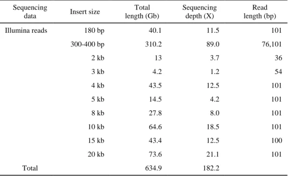
Pepper genome sequences were generated by Illumina platforms (GA2 and Hiseq 2000). PE libraries of 180, 300 and 400 bp were generated with read length of 2x101 bp, 2x76 bp and 2x101 bp, respectively. In case of MP, 2 kb to 20 kb libraries ranging from 2x36 bp to 2x101 bp were sequenced. Total sequences generated by PE and MP sequencing were 350.3 Gb and 284.6 Gb, respectively (Table 1).

To avoid assembly error, we have constructed a pipeline through three-step processes to filter out the low quality and error candidates sequences of pepper genome before assembly. In the first phase, we removed the sequence reads that matched to the released 1,045 bacterial genomes (identity > 98% and coverage > 50%) using CLC Assembly Cell (CLCBio, Denmark). As a second phase, duplicated reads generated by PCR amplification26_{and low-quality sequences were} eliminated by in-house script (Cut-off value: 25 and 20 for PE and MP sequences, respectively). Finally, Quake16 was performed for error correction through the frequency information derived from k-mer graph of sequences using Jellyfish27.

(32)

19

Table 1. Hot pepper genome sequence generated in this study Sequencing

data Insert size

Total length (Gb) Sequencing depth (X) Read length (bp) Illumina reads 180 bp 40.1 11.5 101 300-400 bp 310.2 89.0 76,101 2 kb 13 3.7 36 3 kb 4.2 1.2 54 4 kb 43.5 12.5 101 5 kb 14.5 4.2 101 8 kb 27.8 8.0 101 10 kb 64.6 18.5 101 15 kb 43.4 12.5 100 20 kb 73.6 21.1 101 Total 634.9 182.2

(33)

20

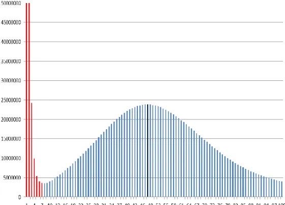
I performed 19-mer analysis for estimation of genome size. All PE reads (180, 300 and 400 bp) were divided into sliding short sequences of 19 bp, overlapping 18 bp except the first base-pair. Using Jellyfish27, the frequency of 19-mers in consideration of both strand was calculated. The 19-mer depth distribution was generated and error candidates with low frequencies of 19-mers were decided. The genome size was estimated as 3.48 Gb by the total volume except low frequencies over the peak of distribution. Low frequency data, indicated as red bar in the Figure 1, were also removed for further assembly.

Insert size of each library is a very important prerequisite for accurate scaffolding. To avoid exaggeration of insert distance and confirm quality of raw data before scaffolding, estimation of insert size for PE and MP was accomplished by reference mapping to the initial contigs from SOAPdenovo17_{. As shown in} Figure. 2, the calculated insert distance of 180, 300, and 400 bp was shown normal distributions indicating the quality of raw data fulfill for genome assembly. In case of MP, ranging from 2kb to 20kb, distribution of insert size for MP also evaluated the raw data as unbiased (Figure 2).

De novo genome assembly and validation

The pre-processed raw sequences were assembled by SOAPdenovo17. To make longer initial contigs, paired reads of the smaller left summit of 180 bp library to each single read were merged by FLASH28. The longer single reads and remained

(34)

21

Figure 1.The 19-mer depth distribution for the raw sequence data of pepper genome. The

19-mer depth distribution shows the information for low frequencies, depth of sequencing and degree of heterozygosity. The X-axis indicates frequency of 19-mer and the y-axis means volume of 19-mer. The red bars in low frequency region are error candidates and the black bar representing sequencing depth is the peak of distribution.

(35)

22

(36)

23

paired reads of PE were assembled as initial contigs using SOAPdenovo without information of the pair. To search optimized k-mer for scaffolding, k-mer size determination was performed using in-house Perl scripts and ‘map’ of SOAPdenovo repeatedly. The best k-mer size of each library for scaffolding was decided independently. Using optimized k-mer of each library, scaffolding was carried out serially until reach to the maximum length of scaffolds. In order to make longer scaffolds, serial scaffolding using SSPACE29_{with strict parameters was} performed with the scaffolds generated by SOAPdenovo. Finally, gaps in the

scaffolds were filled by Gapcloser

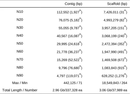
(http://soap.genomics.org.cn/down/GapCloser_release_2011.tar.gz). Total 3.06 Gb (87.9% of the 3.48-Gb total) were assembled into 37,989 scaffolds (N50=2.47 Mb), and 90% of the genome assembly was in 1,276 scaffolds (Table 2 and Table 3). After removing gap sequences, 2.96 Gb of contig sequences were remained (N50=30kb).

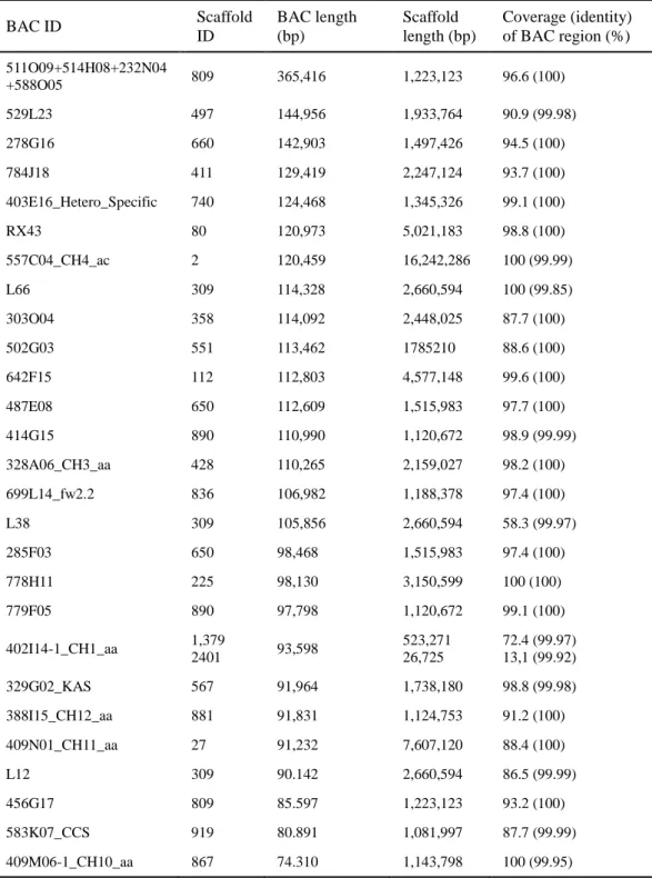
The assembled genome was validated using 27 bacterial artificial chromosome (BAC) single contigs (> 70 kb) generated by ABI and 454 sequencing. BLAST analyses were performed with each BAC clone as a query and scaffolds as subject. The matched regions were selected with a cut-off value of 98% identity and an e-value of 1e-30. Twenty-six BAC sequences were covered by single scaffolds and the assembled scaffolds were matched to all BAC sequences with more than 99.9% identity (Table 3). Although our scaffolds covered most of the regions of BAC

(37)

24

Table 2. Details of CM334 genome assembly

Step Software Insert size (kbp) Raw data coverage (X) N50 (bp) Total number Total size (Gb) Initial contig SOAPdenovo

6,369 866,287 2.53 Scaffold 1 SOAPdenovo 0.18-0.4 100.5 39,971 239,579 2.87 Scaffold 2 SOAPdenovo 2.0 3.7 128,039 123,841 2.90 Scaffold 3 SOAPdenovo 3.0 1.2 167,112 104,553 2.91 Scaffold 4 SOAPdenovo 4.0-5.0 16.7 304,994 74,984 2.94 Scaffold 5 SOAPdenovo 8-10 26.5 562,642 68,781 2.99 Scaffold 6 SOAPdenovo 15-20 38.0 1,300,626 65,751 3.04 Scaffold 7 SSPACE PE + MP 2,472,394 37,989 3.06

(38)

25

Table 3. Statistics of CM334 genome assembly

Contig (bp) Scaffold (bp) N10 112,552 (1,927th) 7,426,011 (31th) N20 76,075 (5,182th) 4,993,279 (82th) N30 55,055 (9,787th) 3,957,205 (151th) N40 40,567 (16,087th) 3,068,199 (240th) N50 29,995 (24,618th) 2,472,394 (352th) N60 21,778 (36,237th) 1,947,990 (491th) N70 15,269 (52,522th) 1,469,508 (672th) N80 9,796 (76,680th) 1,083,843 (915th) N90 4,797 (119,071th) 628,252 (1,276th) Max / Min 442,125 / 71 18,549,843 / 264

(39)

26

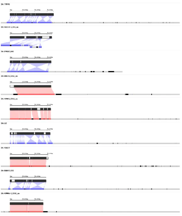
sequences, several low coverage regions were also detected. To confirm the BLAST results for low coverage regions, detailed BLAST results were visualized using an in-house script (Table 4 and Figure 3). As a result, most uncovered regions were confirmed as gap sequences or flanking sequences; however, a few unaligned and inserted regions of the scaffolds were also detected (Figure 3).

Construction and validation of chromosome pseudomolecules

To construct the chromosome pseudomolecules, a high-density SNP map was generated by low-depth (approximately 1X coverage of the genome) whole genome sequencing (WGS) of 120 individual RILs from a cross between Perennial and Dempsey. WGS data was aligned to contigs of the CM334 genome using the Burrows-Wheeler Aligner program (BWA, ver. 0.6.1-r04)30_{. SNPs were detected} using modified default parameters (seed length = 28, maximum differences in the seed =2) and positions of SNPs among aligned reads were identified using SAMtools (ver. 0.1.16)31. SNPs were filtered with parameters (mapping quality = 30, minimum read depth = 3 and maximum read depth = 100). A total of 3,146,751 SNPs between CM334 and Dempsey and 3,160,966 SNP loci between CM334 and Perennial were identified. Qualified SNPs among the three cultivars were determined by filtering non-polymorphic SNPs and heterozygote type loci between Dempsey and Perennial. As a result, 1,798,058 SNPs were identified from 267,173 contigs. Finally, SNPs present in the contigs of less than 10 kb were removed and

(40)

27

Table 4. Summary of validation of the CM334 genome assembly using 27 BAC clones

BAC ID Scaffold ID BAC length (bp) Scaffold length (bp) Coverage (identity) of BAC region (%) 511O09+514H08+232N04 +588O05 809 365,416 1,223,123 96.6 (100) 529L23 497 144,956 1,933,764 90.9 (99.98) 278G16 660 142,903 1,497,426 94.5 (100) 784J18 411 129,419 2,247,124 93.7 (100) 403E16_Hetero_Specific 740 124,468 1,345,326 99.1 (100) RX43 80 120,973 5,021,183 98.8 (100) 557C04_CH4_ac 2 120,459 16,242,286 100 (99.99) L66 309 114,328 2,660,594 100 (99.85) 303O04 358 114,092 2,448,025 87.7 (100) 502G03 551 113,462 1785210 88.6 (100) 642F15 112 112,803 4,577,148 99.6 (100) 487E08 650 112,609 1,515,983 97.7 (100) 414G15 890 110,990 1,120,672 98.9 (99.99) 328A06_CH3_aa 428 110,265 2,159,027 98.2 (100) 699L14_fw2.2 836 106,982 1,188,378 97.4 (100) L38 309 105,856 2,660,594 58.3 (99.97) 285F03 650 98,468 1,515,983 97.4 (100) 778H11 225 98,130 3,150,599 100 (100) 779F05 890 97,798 1,120,672 99.1 (100) 402I14-1_CH1_aa 1,379 2401 93,598 523,271 26,725 72.4 (99.97) 13,1 (99.92) 329G02_KAS 567 91,964 1,738,180 98.8 (99.98) 388I15_CH12_aa 881 91,831 1,124,753 91.2 (100) 409N01_CH11_aa 27 91,232 7,607,120 88.4 (100) L12 309 90.142 2,660,594 86.5 (99.99) 456G17 809 85.597 1,223,123 93.2 (100) 583K07_CCS 919 80.891 1,081,997 87.7 (99.99) 409M06-1_CH10_aa 867 74.310 1,143,798 100 (99.95)

(41)

(42)

(43)

30

Figure 3. Detailed visualization of validation of CM334 genome assembly against 27 BAC

sequences. The upper bars indicate each BAC sequence and the lower bars represent scaffold(s). In BAC sequences, black and white indicate regions matched and unmatched to the scaffold, respectively. In scaffolds, red and blue shading indicate regions matched to the plus and minus strands, respectively. Black intervals represent gap sequences and gray represents unmatched regions of scaffold.

(44)

31

771,587 SNP markers, representing 40,727 CM334 contigs, were used for map construction.

Of 40,272 genetic markers from 40,727 contigs, low-quality markers that contain more than 10% of missing genotype information (10 individuals of 120 RILs) were also removed. Finally, the remaining 21,121 markers were divided into 20 subgroups for genetic map construction (Table 5). To combine each individual genetic map, 180 markers were randomly selected and added to each subgroup, resulting in 1,180 markers in each subgroup. Genetic maps were constructed using Joinmap4 and each genetic map was composed of 11-14 linkage groups (Table 5). To construct a high-density genetic map, 12 identical linkage groups in each genetic map were selected from 20 subgroups based on assignments of 180 commonly used markers in each genetic map. Each linkage group was constructed using selected markers from 12 identical linkage groups, and a high-density genetic linkage map was constructed by combining the individual linkage groups. Finally, a 6,281 marker-containing genetic map, covering 3,796 cM in Kosambi function, was constructed (Table 6).

The pepper chromosome pseudomolecules were built by anchoring scaffolds to a newly constructed high-density genetic map. The pepper genetic map constructed earlier32 was used to increase the accuracy of the pseudomolecule. Markers of the new genetic map were assigned by BLAST to scaffolds with cut-off values of 98% and 80% coverage. The assigned positions of markers were validated

(45)

32

Table 5. Summary of linkage groups from subdivided markers groups

Subgroup # of linkage groups # of markers in linkage group

subgroup01 11 1,092 subgroup02 13 1,046 subgroup03 12 1,042 subgroup04 12 1,057 subgroup05 14 1,065 subgroup06 12 1,053 subgroup07 12 1,022 subgroup08 13 1,079 subgroup09 12 992 subgroup10 12 1,008 subgroup11 13 1,059 subgroup12 13 1,093 subgroup13 12 1,065 subgroup14 12 937 subgroup15 13 1,077 subgroup16 13 1,126 subgroup17 13 1,064 subgroup18 14 1,105 subgroup19 13 1,096 subgroup20 12 1,043 Total 21,121

(46)

33

Table 6. Summary of the integrated 12 linkage groups

Chromosome # markers # selected

markers Genetic distance

# recombination breakpoint 1 1,620 527 468 532 2 1,485 509 493 343 3 1,821 593 375 630 4 1,504 560 427 315 5 1,455 531 254 294 6 2,000 557 223 286 7 1,559 538 287 258 8 540 134 75 54 9 2,143 536 228 242 10 2,826 676 204 224 11 2,652 596 317 350 12 1,516 524 439 333 Total 21,121 6,281 3,796 3,861

(47)

34

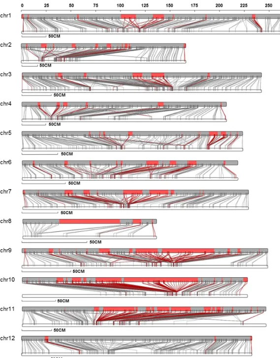
using markers of the earlier genetic map. A total of 4,562 markers from the newly constructed genetic map satisfied the cut-off value, and we were able to anchor 86.0% of scaffolds (2.63 Gb; 1,357 scaffolds) to 12 chromosome pseudomolecules (Figure 4 and Table 7). The direction of scaffolds in 12 chromosomes was determined by considering the ratio of markers shown in identical order in genetic and physical maps using an in-house Perl script. The majority of scaffolds (75.6%) were assigned a direction, and we further assigned the direction of 36 more scaffolds by manual alignment of the unique markers generated from the earlier genetic map.

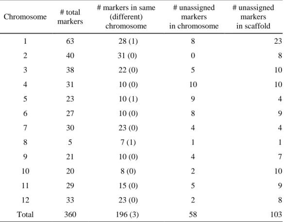
Accuracy of the linkage map was a crucial factor in constructing pseudomolecules. Validation of the genetic map was carried out by checking map reproducibility and by comparison with a previously constructed conserved ortholog set (COS) map33_{. Total 360 COS markers were used for validation except} 10 missed markers and 257 markers were detected in assembled CM334 genome (90% identity, 50% coverage and over 30 bp). As a result, 58 out of 257 markers were appeared in chromosome 0 and 196 out of 199 markers were correctly assigned in 12 chromosomes compared to genetic information (Table 8).

Repeat annotation

Prior to gene prediction, all transposable element-related repeats were masked using REPEATMASKER by masking the genome sequences with the custom library of pepper. The results showed that pepper genome contain approximately

(48)

35

Figure 4. Genetic and physical maps of CM334 genome. The upper bars indicate

pseudomolecules, and the lower bars represent linkage groups corresponding to 12 chromosomes. The grey blocks and lines indicate ordered regions and markers, and the red blocks and lines represent unordered but matched scaffolds to the genetic map.

(49)

36

Table 7. Details of the 12 chromosome pseudomolecules

Chromosome # anchored scaffolds Length of pseudomolecule (bp) # markers # ordered scaffolds (coverage) 1 138 261,560,226 412 120 (86.3%) 2 99 166,118,313 374 85 (84.4%) 3 147 241,745,451 472 130 (86.5%) 4 91 206,470,299 417 81 (91.3%) 5 113 223,151,943 413 91 (89.0%) 6 104 217,864,955 424 83 (82.5%) 7 111 227,551,634 420 85 (73.1%) 8 35 134,909,690 142 21 (47.7%) 9 127 247,983,219 351 81 (58.4%) 10 137 227,301,773 305 65 (43.5%) 11 129 246,428,986 374 89 (60.7%) 12 126 232,591,935 458 117 (97.3%) Total 1,357 2,633,678,424 4,562 1,048 (75.6%)

(50)

37

Table 8. Validation of pseudomolecules using COS markers

Chromosome # total markers # markers in same (different) chromosome # unassigned markers in chromosome # unassigned markers in scaffold 1 63 28 (1) 8 23 2 40 31 (0) 0 8 3 38 22 (0) 5 10 4 31 10 (0) 10 10 5 23 10 (1) 9 4 6 27 10 (0) 8 9 7 30 23 (0) 4 4 8 5 7 (1) 1 1 9 21 10 (0) 4 7 10 20 8 (0) 2 10 11 29 15 (0) 5 9 12 33 23 (0) 2 8 Total 360 196 (3) 58 103

(51)

38

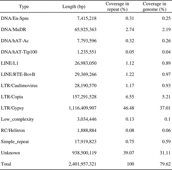
2.34 Gb (76.4%) of TEs and Table 9 reports detail information of transposable elements (TEs) in pepper genome.

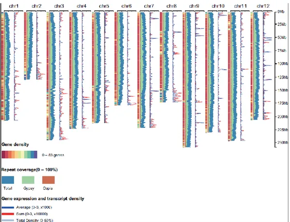
Transposable elements (TEs) have multiple roles in driving genome evolution in eukaryotes34_{. A total of 2.34 Gb (76.4%) of sequences in the assembled CM334} genome was identified as TEs (Table 9). The major type of TE was long terminal repeats (LTRs), which represented approximately 1.7 Gb (more than 70%) of the total number of TEs in the pepper genome. Most of the LTRs were Gypsy elements, which accounted for 67.0% of TEs in CM334, respectively. A large number of Caulimoviridae elements were unique in pepper genome (Table 9). The TEs were widely dispersed throughout the pepper genome and often led to the conversion of euchromatin to heterochromatin. The distribution of the TEs was inversely correlated with the density of genes (Figure 5).

Structural gene annotation

Some gene families containing repetitive sequences (e.g., leucine-rich-repeat (LRR)) sequences such as NB-LRR resistance genes, receptor-like proteins, and receptor-like kinases, had a probability of being recognized as repeat sequences and masked by RepeatMasker. tBLASTn analyses were carried out to prevent masking of genic sequences by repeat masking. Before repeat masking, tBLASTn analyses were carried with protein-coding genes from eight genomes (Arabidopsis thaliana, Solanum lycopersicum, Solanum phureja, Nicotiana benthamiana, Ricinus

(52)

39

Table 9. Classification summary of transposable elements (TEs) of pepper genome

Type Length (bp) Coverage in

repeat (%) Coverage in genome (%) DNA/En-Spm 7,415,218 0.31 0.25 DNA/MuDR 65,925,363 2.74 2.19 DNA/hAT-Ac 7,793,596 0.32 0.26 DNA/hAT-Tip100 1,235,551 0.05 0.04 LINE/L1 26,983,050 1.12 0.89 LINE/RTE-BovB 29,369,266 1.22 0.97 LTR/Caulimovirus 28,190,570 1.17 0.93 LTR/Copia 157,291,528 6.55 5.21 LTR/Gypsy 1,116,409,907 46.48 37.01 Low_complexity 3,034,446 0.13 0.1 RC/Helitron 1,888,884 0.08 0.06 Simple_repeat 17,919,823 0.75 0.59 Unknown 938,500,119 39.07 31.11 Total 2,401,957,321 100 79.62

(53)

40

Figure 5. Global overview of the pepper genome. The global overview of the pepper

genome shows the gene density, coverage of repeats, expression of genes and transcript density at intervals of 1 Mb. Ranging from 0 to 83 genes, and with a genome-wide distribution, gene-rich regions and gene-poor regions are discriminated via colour coding in the 12 chromosomes. The coverage of the repeats represents the proportion of the total TEs and of the Gypsy and Copia elements of LTRs. Gene expression values for total transcriptome except placenta tissues are calculated by the sum of the RPKM (Reads per kb per million reads) and average of RPKM. The transcript density represents the coverage of the total transcriptome, ranging from 0 to 50%.

(54)

41

communis, Vitis vinifera, Glycine max and Populus trichocarpa) to detect putative genic regions. The genome sequences of protein-matched regions was saved as genic regions and recovered as their original sequences instead of being masked. The fraction of the pepper repeat-masked genome with the custom library was 63.28%. No simple repeats, rRNA, tRNA, or microsatellites were masked. This masked genome sequence was used for the pepper genome annotation.

The protein sequences of tomato (iTAG 2.3), potato (PGSC 3.4), grape (Vitis vinifera ver 2.0), Arabidopsis (TAIR10), tobacco (Nicotiana benthamiana, ver 0.4.4), castor bean (Ricinus communis, ver 0.1), soybean (Glycine max, Gmax 109), poplar (Populus trichocarpa, Ptrichocarpa 156), and pepper were mapped using Genewise35 to generate protein-based gene models to determine a consensus gene model. Genewise allows mapping of proteins taking intron-exon boundaries into account. Although the Genewise-predicted pepper gene model was more precise than ab initio programs, Genewise had problems predicting the duplicated genes in pepper the genome. For the annotation of duplicated genes or families of genes, mapping regions of a reference protein in the pepper genome were determined from tBLASTn results using custom Perl scripts. These steps prevented mis-annotation of duplicated or family genes by lacking mapping data of evidence or reference proteins from parsing of single best-matched region from the tBLASTn results in the pepper genome. The Genewise output was reformatted into GFF3 and used as highly reliable data for determining consensus gene model using EVM.

(55)

42

AUGUSTUS21, GENEID20, GlimmerHMM22, and Fgenesh were used for gene prediction in pepper. AUGUSTUS was trained on the pepper genome (release 1.0) using assembled RNA sequences from various tissues (Table 10) and full-length cDNA (GenBank, March 2012). As for preparing the training set for ab initio programs, only predicted pepper cDNAs from TopHat18 and Cufflinks19 whose best hit alignment was at least 50% identical to their best hits and whose length-ratio of subject and query was ≥0.90 were retained as possible full-length pepper proteins. Among these cDNAs, 2000 models were selected and used for generating training sets for gene prediction with GeneID and GlimmerHMM (Table 11).

EVM was used to integrate the various gene models from assembled transcript data, protein data, and ab initio data for determining consensus gene model. To run the EVM, the transcript data, protein data, and ab initio data were converted to EVM-compatible GFF3 format. For conversion, scripts provided by EVM or in-house Perl scripts were used. Genome sequences were then partitioned into smaller data sets to reduce memory requirements, and the sizes of segments were less than 1 Mb. Overlap sizes of partitioned segments were determined using PGA 0.9 version and determined as at least two standard deviations greater than expected gene length. EVM was then run on each of the data partitions, and results of corresponding to partitioned segments were joined into single outputs. Raw output provided by EVM describes the consensus gene structures in a tab-delimited format, listing each exon with the evidence sets that fully support each exon structure.

(56)

43

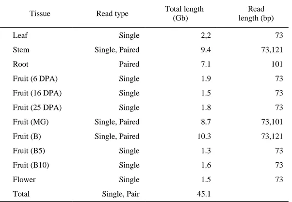
Table 10. Properties of transcriptome used for gene annotation

Tissue Read type Total length

(Gb)

Read length (bp)

Leaf Single 2,2 73

Stem Single, Paired 9.4 73,121

Root Paired 7.1 101

Fruit (6 DPA) Single 1.9 73

Fruit (MG) Single, Paired 8.7 73,101

Fruit (B) Single, Paired 10.3 73,121

Fruit (B5) Single 1.3 73

Fruit (B10) Single 1.6 73

Flower Single 1.5 73

(57)

44

Table 11. Training set for ab initio gene prediction

Average transcript length 1,159 bp

Median transcript length 1,106 bp

Average coding length 886 bp

Median coding length 540 bp

Total length of transcript sequence 1,457,666 bp

Total length of coding sequence 1,279,640 bp

Total exons 1,443 (1.14/gene)

Average exon length 818bp

Median exon length 540 bp

Number of initial exons 256

Average length of initial exons 318 bp

Number of internal exons 748 bp

Average length of internal exon 125 bp

(58)

45

Finally, this raw output was converted to standard GFF3 format. Consensus gene models were validated with tomato and potato proteins (Figure 6). The putative gene models showing longer or shorter gene length compared to tomato or potato genes were validated with the NCBI non-redundant database (NR-DB).

Consensus gene models determined by automatic annotation pipelines mis-annotated genes. To correct these mis-mis-annotated genes, the genomic annotation viewer and editor Apollo (http://apollo.berkeleybop.org/current/userguide.html) was used for error correction. The Apollo program visualizes each gene model used for automatic annotation, such as TopHat/Cufflinks, Genewise gene models from eight genomes, and ab initio gene models, and the user can edit the consensus gene model. Missing or mis-annotated genes were selected from the characterization of each gene family and curated using Apollo. Of the original 35,258 predicted genes, approximately 86 genes were reclassified as pseudogenes and approximately 1,789 genes were discarded in favor of better gene models built by the expert. These manually curated genes were transferred to PGA 1.5 annotation, and the current status reports 34,903 predicted genes, of which 1,789 (3.8%) genes underwent an expert intervention to correct erratic/incomplete gene models (Table 12).

Functional annotation of protein coding genes

To infer functions for the protein-coding genes, we used INTERPROSCAN version 4.836 to scan protein sequences against the protein signatures from InterPro

(59)

46

Table 12. Metrics of pepper gene models

Protein coding Loci (no.) Total CDS length (bp) Avg CDS length (bp) Avg exon length (bp) Avg intron length (bp) Peppera _34,903 _35,247,975 _1,009.9 ₂₈₆ ₅₄₁ Tomatoa _34,771 _35,972,459 _1,057 ₁₇₉ ₅₃₃ Potatob _35,004 _31,678,620 ₉₀₅ ₃₅₆ ₅₉₂ Arabidopsisc _27,206 _24,861,465 _1,212 ₂₆₅ ₁₆₄ Riced _28,236 _78,281,992 _1,081 ₃₁₂ ₄₁₄ a_{The ITAG pre-2.3 pre-release data were used .}

b_{Only protein-coding nuclear transcripts were used.}

c_{All protein-coding transcripts were included, with the exception of TEs and pseudogenes.}

d_{All protein-coding transcripts (MSU Release 6.3) were included, with the exception of TEs, pseudogenes,}

(60)

47

Figure 6. Histogram of pairwise comparison of protein length ratios with their best blast

hit relative to the reference pepper and tomato versus potato. Proteins with a query coverage ratio of 0.9–1.1 can be considered highly confident predictions (43%) because the protein sequences match at the sequence level as well as at the protein length level. Bins of ratios <0.9 are proteins predicted to be shorter than their tomato (iTAG 2.3) reference, while bins of ratios >1.1 indicate proteins predicted to be longer. The zero-bin indicates the number of genes not reporting a hit to the reference given the threshold used. This bin will collect all real species-specific genes and predicted small genes, but also prediction artifacts (false positives = overprediction) or gene models resulting from genome/assembly issues.

0 2000 4000 6000 8000 10000 12000 14000 N umbe r of ge ne s Bin

PGA annotation

_{Pepper vs. Potato} Pepper vs. Tomato Potato vs. Pepper Tomato vs. Pepper

(61)

48

(version 31.0). InterPro integrates protein families, domains and functional sites from different databases, such as Pfam (Ver 24.0), PROSITE (Ver 20.66), PRINTS (Ver 41.1), ProDom (Ver 2006.1), SMART (Ver 6.1), TIGRFAMs (Ver 9.0), PIRSF (Ver 2.74), SUPERFAMILY (Ver 1.73), Gene3D (Ver 3.3.0), and PANTHER (Ver 7.0). INTERPROSCAN integrates the search algorithms of all these databases. INTERPROSCAN identified 193,478 protein domains of 5,544 distinct domain types. Ninety-one percent of the genes (31,566 of a total of 34,903 genes) have been assigned at least one domain. The top 20 SUPERFAMILY domains are plotted in Figure 7.

AGF used similarity searches and lexical analysis for Assignment of Gene Function to protein sequences. It utilized (1) BLASTP37 search results against the Swissprot38_{, TAIR}39_{and TrEMBL}38_{databases and (2) domain search results from} INTERPROSCAN. Query genes matching to genes associated with terms such as “hypothetical protein”, “similarity to” or “predicted protein” were assigned to gene function “unknown”. The highest-scoring description was assigned to the query, and the database accession of the hit protein was added to enable evidence tracking. If INTERPROSCAN results were available, the domain names were extracted and appended to the description line. In case of multiple InterPro matches, the InterPro Parent-Child-tree was used to reduce the number of reported domains by selecting the most specific child and excluding its parents. The descriptions contain, in brackets between the transferred AGF and InterPro domain results.

(62)

49

(63)

50

DISCUSSION

In 2011, the world production value of pepper was 14.4 billion US dollars which was 40 times increased since 19805. Pepper consumption is keep growing every year because of its high nutritional values for human beings. Despite of its increased value, lack of a reference genome sequence has obstructed genomic or genetic research of pepper. In this study, I constructed de novo genome sequence of the pepper as a first reference pepper genome through various processes for preprocessing analysis, assembly, validation and annotation.

Prior to genome assembly, extraction of accurate sequences in huge amount of NGS data is an essential process to minimize assembly error. I performed preprocessing analysis consisted of three steps (1) elimination of prokaryotic genome sequences in the generated raw data, (2) removal of low quality and duplicated reads, and (3) deletion of low frequency region (Figure 8). After preprocessing, as preparation of optimal data for genome assembly and scaffolding, insert sizes of all PE and MP libraries were estimated to construct accurate genomes. Additionally, reads of PE were merged to single reads to make longer initial contigs. Resulting from preprocessing analysis and preparation of optimal data, purified and optimized sequences were prepared for genome assembly.

(64)

51

(65)

52

Until now, general process of assembly and scaffolding have been performed using single assembly tool40-44. In contrast, pepper genome assembly and scaffolding were conducted using firstly SOAPdenovo and then additional scaffolding was carried out using SSPACE to make longer scaffolds. In addition, due to differential account of each library, I performed iterative mapping for each library before scaffolding to obtain optimal values of mer. Using the optimal k-mers for each library, serial scaffolding was conducted. As results, the serial scaffolding process effectively contributed to extend length of scaffolds (Table 2). Furthermore, The genome assembly was validated using 27 bacterial artificial chromosome (BAC) sequences from CM334; 26 BAC sequences were fully covered by each scaffold(s), and showed identities of more than 99.9% (Figure 3 and Table 4).

A distinct difference between completed and draft genome is that whether pseudomolecule construction was performed or not. To construct pseudomolecules, the scaffolds were anchored to a SNP map that was constructed by the sequencing of parental lines and the low depth sequencing of 120 recombinant inbred lines derived from C. annuum cv. Dempsey and C. annuum cv. Perennial. We anchored 86.0% (2.63 Gb, 1,357 scaffolds) of the assembly as 12 chromosome pseudomolecules and ordered them (75.6%) on the basis of genetic distance (Figure x and Table x). Comparing to a previously constructed conserved ortholog set (COS) map33, the validation result revealed that the genetic map correctly assigned the

(66)

53

scaffolds in 12 chromosomes (Table 8).

Although sequencing has become easy, genome-wide annotation of gene structures has become more challengeable due to inaccurate genome assembly generated by short read sequencing45_{. Based on the high quality pepper genome, a} total of 34,903 protein-coding genes were predicted in the PGA pipeline (Pepper Genome Annotation). This gene number is approximately the same as that for tomato (iTAG v2.3, 34,771)46_{and potato (PGSC v3.4, 39,031)}47_{, which suggests a} similar gene number in Solanaceae plants. Overall, 93.2% of the predicted coding sequences were supported by Illumina data, demonstrating the high accuracy of the PGA gene prediction. To validate and improve the gene models, the inaccurately annotated genes were manually curated; 335 genes were manually added and 86 genes were reclassified as pseudogenes. This manual inspection and curation resulted in the replacement of 1,789 genes with better gene models.

Consequently, the pepper genome sequence can serve as an important genomic resource for improving nutritional and pharmaceutical values of pepper as well as support the evolutionary and comparative genomic studies of one of the world-most diversified plant family Solanaceae. The pepper genome sequence provides an excellent tool for exploring the evolution of secondary metabolites in plants. Combined with the recently published tomato46 and potato genomes44 , the pepper genome will elucidate the evolution, diversification, and adaptation of more than

(67)

54

3,000 Solanaceae species, which are adapted to a wide range of geo-ecological habitats ranging from the driest deserts to tropical rainforests.