Doctoral thesis in Medicine
Mortality and Hospital Emergency
Room Visit of Older Adults by
Exposure to Fine Particulate
Matter and Ozone
Graduate School of Ajou University
Department of Medicine
Mortality and Hospital Emergency
Room Visit of Older Adults by
Exposure to Fine Particulate
Matter and Ozone
Prof. Jae-Yeon Jang, Advisor
I submit this thesis as the Doctoral thesis in medicine.
February 2020
Graduate School of Ajou University
Department of Medicine
The Doctoral thesis of En-Joo Jung in Medicine is hereby
approved.
Thesis Defense Committee Chair
Yunhwan Lee Seal
Member Jae-Yeon_Jang Seal
Member Ho-jang Kwon Seal
Member SoonYoung Lee Seal
Member Jae Bum Park Seal
Graduate School of Ajou University
i
Abstract
The effects on particulate matter and ozone on health are being reported by a number of studies. The effects of these air pollutants are likely to be stronger in older adults, but studies in this regard are scarce. The purpose of this study was to study the effects of particulate matter ≤2.5 μm and ozone on acute health effects of older adults.
In order to analyze the health status of older adults, NHIS (National Health Insurance System)-Senior Cohort data and National Statistical Office Mortality records were used. In this study, who were 60 years or older in Seoul, number of ER visit and number of deaths between 2002-2013 were calculated. The current study analyzed each disorder separately and the lag effect. Particulate matter and ozone were analyzed using the single exposure model, as well as the adjusted multi exposure model.
In the single exposure analysis with PM2.5 as the exposure variable, with the increase of 10μg/m3, the number of ER (Emergency Room) visit increased by
1.0062 times, and in the multi exposure model adjusting for meterological factors, the number of ER visit increased by 1.0074 times. There was 1day lag effect and 1.0066 times increase between PM2.5 and ER visit in the multi exposure model, and 1.0057 times when adjusting for ozone (p value <0.10). There was 1day lag effect in all multi exposure models with ozone as the main variable, and when the
ii
particulate matter was adjusted, there was a 1day delay and 1.0143 times increase in ER visit.
In the single exposure analysis with PM2.5 as the exposure variable, with the increase of 10μg/m3, the number of deaths increased by 1.0059 times, and
vascular disease 1.0088 times. In the multi exposure model adjusting for ozone, the number of overall deaths increased by 1.0039 times, and vascular disease 1.0060 times. In the multiple exposure analysis adjusted meterological factors with ozone as the exposure variable, with the increase of 10 ppb, the number of overall deaths increased by 1.0021 times (p value <0.10). There were a 5-day lag effects between PM2.5 and deaths in the multi exposure model, and 1.0032 times when adjusted for ozone.
These results differed depending on the season. Considering the warm and cold period separately, in the multiple exposure model adjusting for ozone, the number of ER visit increased by 1.0210 times were significant in the warm-period due to PM2.5, and in the multiple exposure model adjusting for meterological factors, 1.0323 times were significant in the warm-period due to ozone. In the single exposure model, the overall mortality rate increased by 1.0106 times and mortality due to diabetes increased by 1.0483 times were significant in the warm-period but there were no significant results in the cold-period due to ozone. In association with particulate matters, overall mortality increased by 1.0043 times and mortality due to vascular disease by 1.0063 times in the multiple exposure model adjusted ozone during the cold-period and during the
iii
warm-period, the overall mortality increased by 1.0066 times in the single exposure model.
In this study, an increase in the number of ER visit, and deaths of older adults in accordance with the increase in the PM2.5 and ozone was found. Because the results differed according to warm- and cold- periods, it could be assumed that the period changes the effects of the PM2.5 and ozone on health on older adults. The association found in this study could also influence socioeconomic burden. Future studies need to be performed in regards to younger population, as well as other air pollutants.
iv
Table of Contents
A. List of Text
Abstract... i Table of Contents... iv A. List of Text... iv B. List of Figures... vi C. List of Tables... vi I. Introduction... 1 A. Background………... 1B. Hypotheses and Objectives of Study……….…………... 5
C. Theoretical Review………... 7
1. Vulnerability of Elderly to air pollution... 7
2. Charlson Comorbidity index …………... 8
3. General Characteristics of fine particulate matter and ozone….…10 4. Epidemiologic studies of fine particulate matter and ozone……… 16
II. Methods... 19
A. Study sample & data collection... 20
1. ER visit data... 20
2. Mortality data………... 21
3. Exposure variables... 22
B. Statistical analysis... 24
v
1. Summary statistics of data……… 27
2. Analysis of association between air pollutants and ER visit….… 33 3. Analysis of association between air pollutants and mortality…… 35
4. Analysis of association in period specific outcome………... 37
5. Analysis of association according to lag………... 43
VI. Discussion... 51
1. The influence on ER visit by exposure to air pollutants………... 51
2. The mortality by exposure to air pollutants……… 54
3. Differences of relative risk between ER visit and mortality……….... 58
4. Suggestions and uses of research………. 60
5. Limitation and strength………... 63
V. Conclusion... 65
VI. References... 66
vi
B. List of Figures
▶
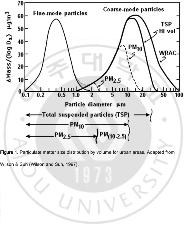
Figure 1. Particulate matter size distribution by volume for urban areas ………. 14▶
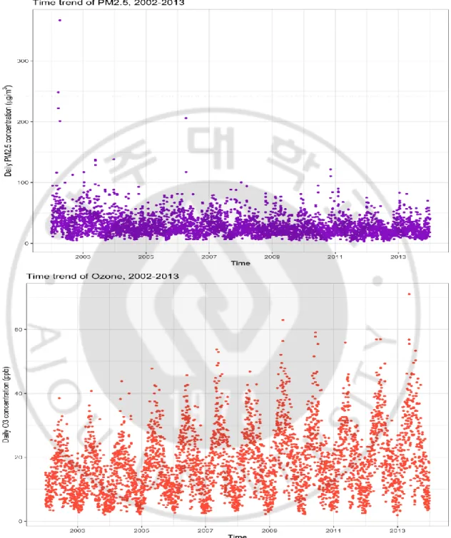
Figure 2. Time trend of PM2.5, ozone concentration in Seoul,2002-2013 ……….……….……… 32
▶
Figure 3. Estimated relative risk (95% interval) in daily ER visit per 10μg/m3 increase in PM2.5 and 10 ppb increase in ozone
concentrations according to lag days……….. 46
▶
Figure 4. Estimated relative risk (95% interval) in daily mortality per 10 μg/m3 increase in PM2.5 and 10 ppb increase in ozoneconcentrations according to lag days……….……….…. 50
C. List of Tables
▶
Table 1. Measures of particulate matter in air………... 15▶
Table 2. Summary statistics of NHIS-Senior Data Base and NationalStatistical Office Mortality records, 2002-2013... 29
▶
Table 3. Summary statistics for daily ER visit and deaths with subgroup of diseases in Seoul, 2002-2013……… 30▶
Table 4. Summary statistics for air pollutants and meterological factors in Seoul, 2002-2013………... 31▶
Table 5. Estimated relative risk (95% intervals) in dailydisease-specific ER visit per 10 μg/m3 increase in PM2.5 and 10 ppb
increase in ozone concentration in Seoul……… 34
▶
Table 6. Estimated relative risk (95% intervals) in dailydisease-specific mortality per 10 μg/m3 increase in PM2.5 and 10 ppb
increase in ozone concentration in Seoul………. 36
▶
Table 7. Estimated relative risk (95% intervals) in daily disease-,period-specific ER visit per 10 μg/m3
increase in PM2.5 and 10 ppb increase in ozone concentration in Seoul……… 38
▶
Table 8. Estimated relative risk (95% intervals) in daily disease-, period-specific mortality per 10 μg/m3 increase in PM2.5 andvii
▶
Table 9. Estimated relative risk (95% interval) in daily ER visit per 10 μg/m3 increase in PM2.5 and 10 ppb increase in ozoneconcentrations in Seoul, according to lag days.………. 44
▶
Table 10. Estimated relative risk (95% interval) in daily mortality per10 μg/m3
increase in PM2.5 and 10 ppb increase in ozone concentrations in Seoul, according to lag days.………. 48
1
I. Introduction
A. Background
High concentrations of fine particulate matter(PM2.5) from automobile
exhaust and a secondary pollutant, ground-level ozone(O3) may cause health problems, and they are associated with increased risk of morbidity and mortality (Buadong et al., 2009; Fann et al., 2012; Hong et al., 2016; Kioumourtzoglou et al., 2017; Orellano et al., 2017; Tallon et al., 2017; To et al., 2016; Zheng et al., 2015). While lots progress has been made in reducing ambient concentrations of air pollution in the Korea, recent levels of PM2.5 and O3 remain elevated from the natural background and are within the range of concentrations found by epidemiology studies to affect health.
In the mid-1980's studies of the deposition and clearance of particles in the respiratory system, along with studies of atmospheric physics and chemistry, suggested that smaller particles might be a larger part of the health threat, and that control strategies should focus on smaller particles. Inhalable particles were defined as particulate matter less than 10 μm aerodynamic diameter (PM10). In the 1990's evidence began to develop suggesting that even smaller particles, that is those less than 2.5 μm
2
(PM2.5), were able to penetrate into the alveolar gas-exchange regions of the lungs, and may be specifically related to health effects (Dockery, 2009). PM2.5: fine inhalable particles, with diameters that are generally 2.5 micrometers and smaller, and originates from construction sites, unpaved roads, fields, smokestacks or fires, including congregated aerosols (e.g. sulfur dioxide, nitrogen dioxide, carbon monoxide, and so on), black carbon (the incomplete combustion of carbonaceous
combustibles) (Zhi et al., 2014), dust, sea salt (Wang et al., 2014), heavy metals, and polycyclic aromatic hydrocarbon (Yoon et al., 2014; Sun and Zhou, 2017).
Ground-level ozone (O3) is formed photochemically in the atmosphere from nitrogen oxides, non-methane volatile organic compounds, methane, and carbon monoxide(Malley et al., 2017). Ozone is a reactive gas
consisting of three oxygen atoms. Its highly oxidizing property defines ozone to be a harmful pollutant when existing in the lower atmosphere. Inhalation of ambient ozone is associated with adverse health
consequences in vulnerable individuals and can lead to exacerbations of pre-existing respiratory diseases such as asthma and COPD (Li et al., 2013). Typical ozone-induced pathophysiological manifestations in humans include immediate decrements in lung function, enhanced airways hyper-reactivity, enhanced epithelial permeability, and inflammation (Que et al., 2011; Li et al., 2013).
Recently, the health effects on elderly has become a principal environmental issue in global, not just in Korea. The elderly are
3
vulnerable to air pollution and show the results of many health effects. There have been studies focusing on the elderly population, in which hospital visit and mortality due to cardiopulmonary disease or asthma were researched (Morgan G, 1998; Téllez-Rojo MM, 2000; Koken et al., 2003; Schwartz et al., 2005; Fann et al., 2012; Di et al., 2017; Orellano et al., 2017; Wheida et al., 2018). Furthermore, similar studies have been conducted in Korea, in which the associations between air pollutants with depression and insulin resistance (Kim and Hong, 2012; Lim et al.,
2012b), as well as acute stroke death were found (Hong, 2002).
Previous studies considering the relationship between air pollution and elderly health have used time series analysis (Goldberg, 2001; Wong CM, 2002; Martins LC, 2006; Cakmak et al., 2007; Kan et al., 2008;
Szyszkowicz, 2008; Carlsen, 2013), often using fine particulate matter and ozone as exposure variables, and hospital visit or mortality as the
outcome variable.
Despite the importance of prior studies, they have been limited to specific illnesses such as cardiovascular or respiratory diseases, and all- cause mortality. Moreover, studies considering the association of health effects, fine particulate matter and ozone among Korean elderly using national big database is scarce, especially, few studies have been
conducted to investigate air pollutants and health effects in Korean elderly using both emergency room visit and deaths as outcome variables. Our study aimed to study the effects of fine particulate matter and ozone on the health of community-dwelling elders in Seoul area using
NHIS-4
Senior Cohort data and National mortality data of the Korea National Statistical Office. Furthermore, additional analysis was conducted to distinguish between illnesses, as a cause of health effects, and different models taking into account various lag period were postulated to assess possible delayed effects.
5
B. Hypotheses and Objectives of Study
The hypotheses of this study are as follows:
First, the health effects of fine particulate matter and ozone are different. Previous studies have shown that particulate matter and ozone have different impact mechanisms, which may lead to differences in health effects.
Second, fine particulate matter and ozone will affect health effects on elderly.
Previous studies have considered particulate matter and ozone in terms of health effects, but studies in the vulnerable elderly population are scarce.
Third, fine particulate matter and ozone will affect specific illnesses differently.
Previous studies have been studies focusing on the effects of air pollutants, in which emergency room visit and mortality due to cardiovascular or respiratory diseases. Despite the importance of prior studies, they have been limited to specific illnesses such as above, or all-cause results.
Fourth, fine particulate matter and ozone will have different health effects according to season.
6
pollutants at different season by temperature, but the results were inconsistent.
Fifth, fine particulate matter and ozone will have different lag effects according to variant medical services.
Previous studies have reported lag effects in the health impacts of air pollutants, however, the results have been analyzed individually by medical institution. In contrast, this study will show how the lag effects of medical care or death differ.
The purpose of this study were to study the effects of fine particulate matter and ozone the health of community-dwelling elders in Seoul area using NHIS-Senior Cohort data and death data of the Korea National Statistical Office. Health effects were identified as outcome variables for emergency room visit, and death. Furthermore, additional analysis was conducted to distinguish between illnesses, as a cause of health effects, and different models taking into account various lag days and were postulated to assess possible lag effects and period-specific effects to assess changes by season.
7
C. Theoretical Review
1. Vulnerability of Elderly to Air Pollution
The very young and very old are easily identifiable subgroups of interest, because they are well-recognized as a susceptible
subpopulation. During the early periods of life, air pollution has been associated with preterm birth, intrauterine growth retardation, sudden infant death syndrome, and infant mortality (Wang X, 1997; Ritz et al., 2002; Ha et al., 2003; Liu et al., 2003; Dales R, 2004). Among the elderly, adverse effects on hospital admission of air pollution have been reported in those > 65 years of age (Schwartz, 1994). The increased vulnerability of the elderly against air pollutants was also shown in a previous study, in which the mortality rate due to air pollutants was 2-3 times higher for those 85 or older compared to those 65 and younger (Cakmak et al., 2007).
In older adults, long-term exposures have been negatively associated with lung function (Trenga et al., 2006; Lee et al., 2007; Alexeeff et al., 2008; Forbes et al., 2009) and positively associated with respiratory symptoms (Höppe et al., 2003; Schikowski et al., 2010). Furthermore, in terms of the vulnerability to particulate matter in the elderly could be explained through three mechanisms: 1) A reduced physical reserve due to the body’s response to counter-act the harmful effects of particulate
8
matter; 2) Increased inflammation due to particulate matters; 3) Weakened health due to sarcopenia (Eckel et al., 2012).
That’s why we should investigate the possibility of vulnerable elderly, and there is an importance to understand for health effects of the
subpopulation and to make a proper guidance of air quality standards.
2. Charlson Comorbidity Index
The Charlson comorbidity index (Charlson et al., 1987), a method of predicting mortality by classifying or weighting comorbid
conditions(comorbidities), has been widely utilized by health researchers to measure burden of disease and case mix (Quan et al., 2011).
Since the publication of Charlson et al.’s original article in 1987 (Charlson et al., 1987), the index has been validated for its ability to predict mortality in various disease subgroups, including cancer, renal disease, stroke, intensive care, and liver disease (Poses et al., 1996; Hemmelgarn et al., 2003; Goldstein et al., 2004; Lee et al., 2005; Baldwin et al., 2006; Myers et al., 2009; Quach et al., 2009; Quan et al., 2011).
9
the index after a review of 559 hospital charts for patients admitted to medical services at 1 hospital and then assessed the association of these comorbidities with 1-year all-cause mortality (Charlson et al., 1987). Among many potential comorbidity variables assessed, 17 were found to be associated with 1-year mortality. To measure disease burden,
Charlson et al. assigned a weighted score to each comorbid condition based on the relative risk of 1-year mortality. After validating the index in breast cancer patients, Charlson et al. reported that the score as an indicator of disease burden had a strong ability to predict mortality
(Charlson et al., 1987). To apply the index in administrative hospital discharge data, Deyo et al. (Deyo RA, 1992), Romano et al. (Romano et al., 1993), and D’Hoore et al. (D'Hoore et al., 1996) independently developed coding algorithms using the International Classification of Diseases, Ninth
Revision (ICD-9), and its clinical modification (ICD-9-CM). Later, Quan et al. (Quan H, 2005) developed International Classification of Diseases, Tenth Revision (ICD-10), coding algorithms to define the Charlson index, and Sundararajan et al. (Sundararajan et al., 2007) assessed the index’s performance in ICD-10 international hospital discharge abstract
databases(Quan et al., 2011).
In this study, the number of daily overall as well as disease-specific ER visit and mortality incidents were analyzed. In terms of the disease-specific incidents, illnesses such as vascular disease, chronic respiratory disease, diabetes and hypertension were classified according to the Charlson Comorbidity Index (CCI) based on the International
10
Classification of Diseases (ICD-10).
3. General Characteristics of Fine Particulate matter and
Ozone
Inhalable irritants include both gas and solid phase air pollutants such as particulate matter and ozone.
The term particulate matter refers to solid or liquid particles in the air. Particulate matter has many sources and can be either primary or
secondary in origin. Primary particulate matter is emitted directly and can be either coarse or fine, whereas secondary particulate matter, which tends to be finer in size, is formed in the atmosphere through physical and chemical conversion of gaseous precursors such as nitrogen oxides
(NOx), sulfur oxides (SOx), and volatile organic compounds (VOCs). Whereas most air pollutants are defined with respect to a particular chemical composition, particulate matter is a generic term that includes a broad range of physical characteristics and chemical species (Bell et al., 2004).
For regulatory and scientific purposes, particulate matter is measured according to the mass concentration within a specific size range(Wilson and Suh, 1997; Bell et al., 2004) (Figure 1 and Table 1). Size
11
transportation, environmental deposition, and the pattern of deposition in the respiratory system. Particle size is characterized by aerodynamic diameter, which is the diameter of a uniform sphere of unit density that would attain the same terminal settling velocity as the particle of interest. This measure facilitates size comparison among irregularly shaped
particles and refers to the physical behavior of the particles rather than the actual size.
For regulatory and research purposes, several different particle metrics have been used (Bell et al., 2004) (Table 1). Thus, the various fractions of particulate matter in air have been defined and measured without regard to their composition, to date. Particles in the air can be characterized both physically and chemically. In typical urban environments, there are two broad sets of source categories: (a)
combustion sources, including mobile sources (predominantly vehicles) and stationary sources (primarily industrial sources and power plants); and (b) mechanical forces, including wind, and vehicle traffic and other activities (Bell et al., 2004). The smaller particles result from combustion and stationary sources, whereas the larger particles tend to come from mechanical forces, such as wind or road traffic. Particles in urban air tend to have a multimodal distribution, reflecting these sources(Wilson and Suh, 1997; Bell et al., 2004) (Figure 2). In a sample of urban air, coarse particles typically make up a small fraction of all particles with regard to number density but comprise a large fraction with respect to volume or mass. Smaller particles contribute less to total volume and mass but more to surface area and the total number of particles. In recent health effects
12
research, emphasis has been placed on the smaller particles because they are in the size range that penetrates into the lung without being removed in the upper airway (EPA, 2004).
Ozone, a highly reactive gas and major component of urban smog, is formed in the presence of sunlight from the interaction of volatile organic compounds with oxides of nitrogen, both of which are generated from multiple sources, for example, motor vehicle exhaust, industrial emissions, gasoline vapors, and chemical solvents. In addition, photooxidative aging of airborne emission mixtures enhances toxicity of respirable particulates (Sexton et al., 2004; Bosson et al., 2008; Que et al., 2011).
An edemagenic lung irritant like ozone can deposit on epithelial membrane surfaces of the airway and also penetrate to the more distal surfaces essential for gas exchange (Hu et al., 1994). Toxicity of ozone to respiratory tissues is primarily attributed to generation of reactive oxygen metabolites and ozononation of fatty acids present at epithelial cell
surfaces and in lung lining fluids (Leikauf GD, 1995; Pryor et al., 1995). In controlled laboratory settings, early (3 h)and late (1-day post)
responses of human subjects to O3 exposure include an infiltration into airway and alveolar surface fluids of serum proteins, inflammatory cells, and mediators (Koren et al., 1989; Devlin et al., 1996). The presence of cellular and molecular markers of epithelial membrane injury and the diffusivity of small hydrophilic molecules within submucosal tissues suggests epithelial injury together with soluble cellular and secreted mediators likely contribute to enhancement of physiological and airway
13
functional responses, i.e., airway hyperreactivity (Seltzer J, 1986; Que et al., 2011).
An alteration of epithelial integrity conveys a risk that xenobiotic and mitogenic substances that are normally contained by barrier defenses at epithelial surfaces may gain access to submucosal tissue elements leading to injury and increases in tissue repair (Teisanu et al., 2011). Also, it was determined that airway hyperresponsiveness in response to nonspecific bronchoprovocation was also present at ∼1-day postexposure, although a range in severity of the airway hyperreactivity was codependent on environmental temperature conditions of the exposure to ozone (Foster WM, 2000). Airway hyperresponsiveness is present in all humans with asthma, at least when symptomatic. The long-term effects of increased airway responsiveness are considered as a risk factor for the
14
Figure 1. Particulate matter size distribution by volume for urban areas.Adapted from Wilson & Suh (Wilson and Suh, 1997).
15 Table 1. Measures of particulate matter in air
Particle metric Definition
Black smoke or British smoke (BS)
A nongravimetric measure in which air is passed through a filter paper and the darkness of the resulting stain is determined
Coefficient of haze (COH)
Measure of the intensity of light transmitted through a filter with particles relative to that of a clean filter
Total suspended particles (TSP)
Particles with an aerodynamic diameter up to approximately 45 microns
PM10 Particles with an aerodynamic diameter no larger than 10 microns PM2.5 Particles with an aerodynamic diameter no larger than 2.5 microns Ultrafine Particles with an aerodynamic diameter no larger than 0.1 microns Adapted from Bell, et al (Bell et al., 2004).
16
4. Epidemiologic Studies of Fine Particulate Matter and
Ozone
In the past, a number of studies have considered particulate matter and ozone in terms of morbidity and mortality (Linn, 2000; Ensor et al., 2013; Shields KN, 2013; Yamazaki et al., 2014; Hao et al., 2015; To et al., 2016; Tallon et al., 2017). There have also been studies focusing on the effects of air pollutants on the elderly population, in which hospital visit (e.g., inpatient or outpatient) and mortality due to cardiopulmonary disease or asthma were researched (Morgan G, 1998; Téllez-Rojo MM, 2000; Koken et al., 2003; Schwartz et al., 2005; Fann et al., 2012; Orellano et al., 2017; Wheida et al., 2018). Some studies have identified ambient air pollutants ozone and particulate matter as the main exposures in a study. According to a study published in Thailand in 2009, exposure on the previous day to PM10 and O3 had a positive association with hospital visit for CVD
(cardiovascular diseases) among elderly (≥65 years) individuals. The increase in CVD hospital visit in this age group was 0.10% with a 10 µg/m3 increase in PM10, and 0.50% with an increase in O3 (Buadong et al., 2009). A study published in 2017 identified the association between air pollution and onset of depression in middle-aged women, hazard ratios for both pollutants were elevated (per 10ppb increase in ozone, hazard ratio (HR) = 1.06; per 10 μg/m3 increase in 1-year PM2.5, HR = 1.08
(Kioumourtzoglou et al., 2017). Other study has identified the association between air pollution and erectile dysfunction (ED) in men over 57 years of age, they found positive, associations between PM2.5, O3 exposures
17
and odds of incident ED, and observed associations were robust to model specifications and were not statistically significant by any of the examined risk factors for ED (Tallon et al., 2017). Also, a study published for to determine if individuals with asthma exposed to higher levels of air
pollution have an increased risk of asthma–chronic obstructive pulmonary disease (COPD) overlap syndrome(ACOS), the adjusted hazard ratios of ACOS and cumulative exposures to PM2.5 (per 10 mg/m3) and O3 (per 10 ppb) were 2.78, and 1.31, respectively (To et al., 2016).
Furthermore, several studies have been conducted in Korea, in which the associations between air pollutants with depression and insulin resistance (Kim and Hong, 2012; Lim et al., 2012b), as well as acute stroke death were found (Hong, 2002).
Previous studies considering the relationship between air pollution and elderly health have used time series analysis (Goldberg, 2001; Wong CM, 2002; Martins LC, 2006; Cakmak et al., 2007; Kan et al., 2008;
Szyszkowicz, 2008; Carlsen, 2013), often using particulate matter and ozone as exposure variables, and morbidity or mortality as the outcome variable.
A time series is a sequence of measurements equally spaced through time or along some other metameter. Time series data are naturally
generated when a population or other phenomenon is monitored over time. The daily number of live births or deaths, the monthly average
temperature, the annual Medicare expenditures over many years are all examples of time series. Most often in public health and biomedical
18
research, the objective of research is to understand how explanatory variables influence an outcome over time so that regression analysis is used (Zeger et al., 2006).
In 2003, Fisher et al. used the mortality record in Netherlands and found associations between pm10, pneumonia and mortality as well as in regards to ozone, cardiovascular problems, pneumonia and mortality in people 75 years or older (Fischer et al., 2003). Also, in a study published by Goldberg et al. in 2013 found that people, aged 65 years or older, with a history of heart failure or atrial fibrillation had and increased mean percent change of mortality due to PM2.5, and those with a history of coronary artery disease had an increased mean percent change of mortality due to ozone (Goldberg et al., 2013). Furthermore, Di et al. reported in 2017 that an increase of 10 μg/m3 in PM2.5 and 10 ppb in
warm-season ozone were statistically significantly associated with a relative increase in all-cause daily mortality rate (Di et al., 2017).
Also, previous studies considering the relationship between air pollution and elderly health have published, using hospital visit as the outcome variable. In 2012, Winquist et al. reported using hospital records in Missouri, USA that visit of emergency room or hospitalizations due to respiratory illnesses was affected by air pollutants (Winquist A, 2012). Wang et al. used data from a hospital in Shanghai, China in 2018 and found that fine particulate matter increased outpatient visit due to respiratory illness in older people aged 60 and over (Wang et al., 2018). According to a research paper published in 2015, the number of hospital visit and hospitalizations for asthma in elderly people increased due to particulate
19
matter and ozone (Zheng et al., 2015). A meta-study published in 2017, which used studies following a case-crossover design with records of emergency departments and/or hospital admissions as a surrogate of moderate or severe asthma exacerbations were selected, both PM2.5 and ozone were associated with asthma exacerbation. (Orellano et al., 2017).
Despite the importance of prior studies, they have been limited to specific illnesses such as cardiovascular or respiratory diseases.
Moreover, studies considering the association of ER visit or mortality, fine particulate matter and ozone among Korean elderly using national
20
II. Methods
A. Study sample & data collection
1. ER visit data
The study was analyzed using an NHIS-Senior built in the National Health Insurance System (NHIS). The elderly cohort was constructed by randomly extracting 558,147 of approximately 5.5 million elderly
subscribers over 60 years of age to identify risk factors of senile diseases and analyze their prognosis and included information such as
socioeconomic variables, medical history, and health examination results. Almost all Koreans are affiliated with the National Health Insurance
System, and their medical use records are managed by the NHIS, which is representative of Korea's elderly population. I used this elderly cohort to analyze those who live in Seoul and have experienced emergency room visit from 2002 to 2013. The number of emergency room visit per day of the study period was calculated and used as the outcome variable. If a subject visit emergency room several times during the study period, the number of emergency room visit is added to the corresponding emergency room visit, and if more than one visit was treated as one case. The total number of emergency room visit in this study was 39,464 patients. The number of emergency visit during the study period and the number of sample subjects are shown in Table. 2.
The number of daily overall as well as disease-specific ER visit were analyzed. In terms of the disease-specific morbidity, illnesses such as
21
vascular disease, chronic respiratory disease, diabetes and hypertension were classified according to the Charlson Comorbidity Index (CCI) based on the International Classification of Diseases (ICD-10). In regards to vascular disease, myocardial infarction (I21.x, I22.x, 125.2), congestive heart failure (I09.9, I11.0, I13.0, I13.2, I25.5, I42.0, I42.5-I42.9, I43.x, I50.x, P29.0), peripheral vascular disease (I70.x, I71.x, I73.1, I73.8, I73.9, 177.1, 179.0, I179.2, K55.1, K55.8, K55.9, Z95.8, Z95.9), and cerebrovascular disease (G45.x, G46.x, H34.0, I60.x-I69.x) were included. Also, (127.8, 127.9, J40.x-J47.x, J60.x-J67.x, J68.4, J70.1, J70.3) for chronic respiratory disease, both diabetes without other complications and with other complications (E10.x-E14.x) were included (Quan H, 2005). Lastly, although hypertension is not included in CCI, because it is a highly prevalent disease in the Korean elderly population (Kim and Kim, 2015), it was included in the study with the classification of I10.x.
The data in this study were anonymized, non-personalized and retrospective and did not receive individual consent from the subjects. The study was approved by Ajou University Hospital for IRB approval (Approval no.: AJIRB-SBR-EXP-18-494).
2. Mortality data
Current study utilized the mortality data from Korean National
Statistical Office to analyze the mortality data of those 60 years or older living in Seoul area between 2002 to 2013. Daily mortality incidents during the study period were collected and used as the outcome variable measure. Because more than 95% of the death certificates in Seoul are
22
completed by medical doctors, these reports are assumed to be credible. There were 343,968 overall mortality incidents and 28,664 yearly
mortality incidents during the study period. The number of deaths during the study period are shown in Table 2. and the overall as well as disease-specific number are shown in Table 3.
The number of daily overall as well as disease-specific mortality incidents were analyzed. In terms of the disease-specific mortality, illnesses such as vascular disease, chronic respiratory disease, lung cancer, diabetes and hypertension were classified according to the Charlson Comorbidity Index (CCI) based on the International
Classification of Diseases (ICD-10), and ICD-10 codes included by disease are the same as medical services data.
The data in this study were anonymized, non-personalized and retrospective and did not receive individual consent from the subjects. The study was approved by Ajou University Hospital for IRB approval (Approval no.: AJIRB-SBR-EXP-19-327).
3. Exposure variables
Both PM 2.5 and ozone level were measured hourly. The amount of particulate matter was measured using ‘Beta-ray absorption method’, which measures the amount of beta-ray absorbed by a certain substance, considering the characteristic of the beta-ray being absorbed more in bigger substances.
To measure the ozone level, an ultraviolet ray with the wavelengths of 253.65nm, which is most easily absorbed by the ozone, was shot at the ozone. The amount of the beta-ray, which was absorbed by the ozone and
23
decreased, was measured to calculate the ozone level. The amount of PM 2.5 from 2002 to 2013 was acquired through the Climate Environment Division of Seoul, and the ozone level as well as other weather factors were acquired through the Ministry of environment. The daily average of PM2.5 and ozone measurements were analyzed with meterological factors (e.g., daily average of temperature, atmospheric pressure, and humidity) to account for other weather variation.
24
B. Statistical analysis
The number of disease-specific daily ER visit incidents, death and 2 air pollutants (e.g., particulate matter and ozone) were recorded according to date, and analyzed by the time series method. More detailed information regarding the statistical model is described in a previous study(En-Joo Jung, 2019). In this study, a single exposure model (i.e., air pollutants were treated as single air pollutant) and a multiple exposure model (i.e., each air pollutant was adjusted for the other air pollutant) were used. The purpose of using these models was to ascertain whether or not the
association between an air pollutant and outcome remained significant even after adjusting for the other air pollutant. For example, in a single exposure model in terms of the particulate matter only included the effect of the particulate matter, but the multiple exposure model was able to account for the effects of both the particulate matter and ozone. Air pollutants such as sulfur dioxide or nitrogen dioxide were not included in the current study, because according a previous study(En-Joo Jung, 2019), adjusting for these factors decreased the statistical power in regards to PM2.5, and a strong correlation between the main exposure variable (e.g., PM2.5) and sulfur dioxide or nitrogen dioxide. Because the overall mortality and hospital visit rate was close to a Poisson distribution, and the explanatory variables of mortality were mostly nonlinear, the Generalized Linear Model (GLM) was used. In this model, the main exposure variable was the daily average of each air pollutant level. GLM combines the time series analysis, Poisson distribution and natural spline
25
to calculate the short-term relationship between particulate matter, ozone and disease-specific mortality and hospital visit. The Partial
autocorrelation function was used to induce the optimal degrees of freedom (df) in the natural spline of the calendar time, which was 4 per year according to Peng(Dominici and Peng, 2008). Therefore, the season and long-term trend was controlled for by the natural 3rd smooth spline with the calendar time (df = 4 * 12). Considering previous studies(Lim et al., 2012a; Xu, 2014), temperature and other pollutants (df=3) at the time of mortality incident were integrated in to the natural 3rd smooth spline model. Day of the week (DOW), which was a categorical variable, was used as a dummy variable to control for all DOW related variables. The final model is shown below.
log[𝐸(𝑌𝑡−𝑖)] = 𝛼 + 𝛽1𝑃𝑀2.5𝑡−𝑖 𝑜𝑟 𝛽1𝑂3𝑡−𝑖+ 𝑛𝑠 (𝑇𝑒𝑚𝑝0, 𝑑𝑓 = 3) + 𝐻𝑢𝑚𝑖 + 𝑃𝑟𝑒𝑠𝑠
+ 𝑛𝑠 (𝑃𝑀2.50 𝑜𝑟 𝑂30, 𝑑𝑓 = 3) + 𝑛𝑠 (𝑇𝑖𝑚𝑒, 𝑑𝑓 = 4 ∗ 12) + 𝛽2𝐷𝑂𝑊
E(Y t-i) is the expected number of ER visit incidents and deaths;
PM2.5t-i and O3t-i are the average amount of PM2.5 and ozone level in
Seoul with i being the lag day; ns is the natural 3rd spline; Temp0 is the
daily average temperature (° C), Humi is the daily relative humidity (%), and Press is the daily relative atmospheric pressure (hPa); PM2.50 and
O30 are the densities of PM2.5 and ozone; Time indicated the long-term
trend as well as seasonal effects with calendar days; DOW indicates the day of the week.
Considering the lag model, in which the resulting effect is delayed compared to the exposure, the model consists a delay (lag). For example, lag1 indicates an exposure a day prior to the resulting incident. Different
26
lag effects were observed in prior studies. In terms of ischemic stroke, a latency between 0 and 1 was apparent (i.e., the day of as well as a day prior to the exposure)(Ca et al., 2007), for chronic obstructive pulmonary disease, a latency of 0-3 (i.e., the day of, as well as one day, two days and three days prior to the exposure)(Fung et al., 2006), and in terms of cardiovascular mortality and morbidity, a latency of 1-5 days was
observed(Halonen et al., 2010). With a careful consideration of prior results, the current study analyzed a latency up to 5 days making a single lag model (lag0 ~ lag5). Disease-specific relative risks were described according to the day of the exposure (Table 5~ 10).
To analyze the seasonal different effects of air pollution on mortality and ER visit, study periods were divided into warm periods and the rest into cold periods. Based on average temperature, considering June to August as warm-period and the rest as cold-period. The association between air pollutants and daily relative risk differed depending on the season. Period-specific rate was described with disease-specific rate (Table 7~8).
The results of the statistical analysis in the current study were based on the relative risk of daily ER visit and mortality due to 10 ㎍/㎥
increase in the fine particulate matter density and 10 ppb increase in the ozone density. A p-value below 0.05 was considered statistically
significant, and all analyses were conducted using R statistical software, Version 3.3.3.
27
III. Results
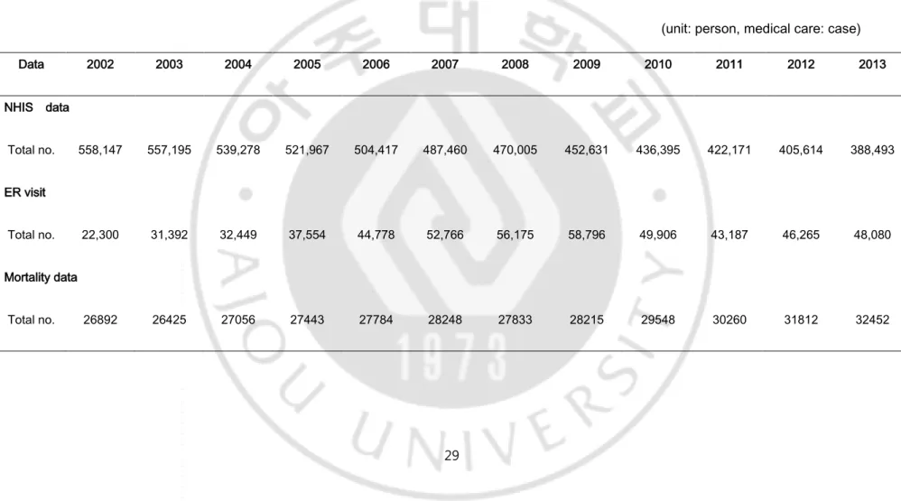
1. Summary statistics of ER visit, deaths and air pollutants data Table 2 summarizes statistics of data of NHIS-Senior Data Base and National Statistical Office Mortality records from 2002 to 2013.
The elderly cohort was built in 558,147 in 2002 and has been in the form of a cohort with no personnel. As a result, the total number of subjects decreased every year, and in 2013 it was 388,493. The availability of emergency room visit varies from year to year and has increased since 2009, and has since declined. The total number of deaths by year also varies from year to year, but shows a relatively similar trend until 2008, with an increase thereafter.
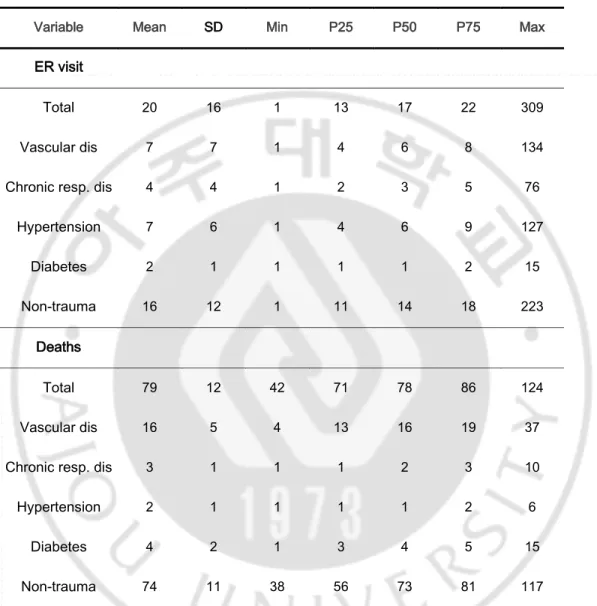
Table 3 summarize statistics of daily ER visit and deaths from 2002 to 2013.
The average daily ER visit within same period was 20, with range of 16 to 309 visit per day. The average number of non-traumatic visit was 16 visit per day.
The average daily death toll within same period was 79, with range of 12 to 124. The average number of non-traumatic deaths was 74 persons per day. The mean number of deaths from vascular diseases was 16 and the mean number of deaths from chronic respiratory diseases was 3.
28
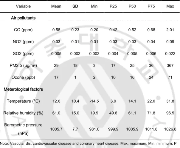
Table 4 summarize statistics for air pollutants and meterological factors from 2002 to 2013.
The average PM2.5 level during this period was 29g/m3and the highest
density was 367 g/m3, at a minimum of 3 g/m3, and the average Ozone
level was 17 ppb and the highest density was 71 ppb, at a minimum of 2 ppb. The average concentration of CO was 0.58 ppm and the average concentration of NO2 was 0.03 ppm,and the average concentration of SO2 was 0.005 ppm. 1 ppb corresponds to a concentration equal to 1000 ppm and this study results in a 10 ppb increase.
The mean daily temperature over 12 years was 12.6℃, and the
temperature ranged from -14℃ to 31.8℃. The relative humidity was 61% on average, and the average barometric pressure was 1005.7 hPa.
Figure 2 shows the time trend of PM2.5 and ozone in Seoul from 2002 to 2013. Seasonal changes in concentrations of both air pollutants occur, and ozone shows an increase in peak concentrations in the mid to late 2000s, and no significant changes have been found since, while PM2.5 generally decreases.
29
Table 2. Summary statistics of NHIS-Senior Data Base and National Statistical Office Mortality records, 2002-2013.
(unit: person, medical care: case)
Data 2002 2003 2004 2005 2006 2007 2008 2009 2010 2011 2012 2013 NHIS data Total no. 558,147 557,195 539,278 521,967 504,417 487,460 470,005 452,631 436,395 422,171 405,614 388,493 ER visit Total no. 22,300 31,392 32,449 37,554 44,778 52,766 56,175 58,796 49,906 43,187 46,265 48,080 Mortality data Total no. 26892 26425 27056 27443 27784 28248 27833 28215 29548 30260 31812 32452
30
Table 3. Summary statistics for daily ER visit and deaths with subgroups of disease in Seoul, 2002-2013.
Variable Mean SD Min P25 P50 P75 Max
ER visit
Total 20 16 1 13 17 22 309
Vascular dis 7 7 1 4 6 8 134
Chronic resp. dis 4 4 1 2 3 5 76
Hypertension 7 6 1 4 6 9 127 Diabetes 2 1 1 1 1 2 15 Non-trauma 16 12 1 11 14 18 223 Deaths Total 79 12 42 71 78 86 124 Vascular dis 16 5 4 13 16 19 37
Chronic resp. dis 3 1 1 1 2 3 10
Hypertension 2 1 1 1 1 2 6
Diabetes 4 2 1 3 4 5 15
Non-trauma 74 11 38 56 73 81 117
Note: Vascular dis, cardiovascular disease and coronary heart disease; Max, maximum; Min, minimum; P, percentile; Chronic resp. dis, chronic respiratory disease; SD, standard deviation.
31
Table 4. Summary statistics for air pollutants and meterological factors in Seoul, 2002-2013.
Variable Mean SD Min P25 P50 P75 Max
Air pollutants CO (ppm) 0.58 0.23 0.20 0.42 0.52 0.68 2.01 NO2 (ppm) 0.03 0.01 0.01 0.03 0.03 0.04 0.09 SO2 (ppm) 0.005 0.002 0.002 0.004 0.005 0.006 0.022 PM2.5 (μg/m3) 29 18 3 17 25 36 367 Ozone (ppb) 17 1 2 10 16 24 71 Meterological factors Temperature (°C) 12.6 10.4 -14.5 3.9 14.1 22.0 31.8 Relative humidity (%) 61.0 15.0 19.9 49.6 61.1 71.8 96.5 Barometric pressure (hPa) 1005.7 7.7 981.0 999.9 1005.9 1011.8 1026.8
Note: Vascular dis, cardiovascular disease and coronary heart disease; Max, maximum; Min, minimum; P, percentile; Chronic resp. dis, chronic respiratory disease; SD, standard deviation.
32
33
2. Analysis of association between air pollutants and ER visit
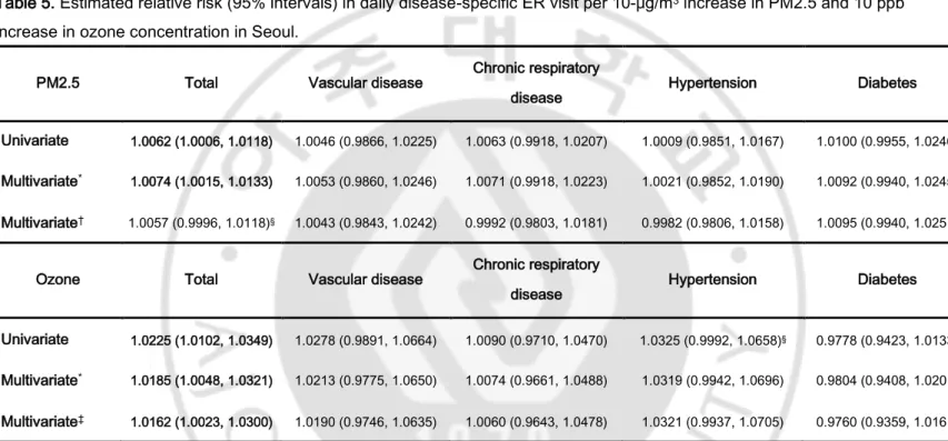
Table 5 estimated relative risk of ER visit with increase in PM2.5 and ozone.
The relative risks expected in daily emergency room visit increased by 1.0062 times (95% CI 1.0066-1.0118, p <0.05) as the fine particulate matter increased by 10 ㎍/㎥ in the single exposure model and 1.0074 times (95% CI 1.0015-1.0133, p <0.05) in the model adjusted meterological factors. Increasing PM2.5 concentrations were also associated with an increase in emergency visit due to total disease in ozone-adjusted multiple exposure model (1.0057 times, 95% CI 0.9996-1.0118, p <0.10). As the concentration of ozone increased by 10 ppb, it was 1.0225 times (95% CI 1.0102-1.0349, p <0.05) in the single exposure model of total disease, and 1.0185 times in the multiple exposure model adjusted meterological factors (95% CI 1.0048-1.0321, p <0.05) and ozone increased 1.0162 times (95% CI 1.0023-1.0300, p <0.05) in the PM2.5 adjusted multiple exposure model.
34
Table 5. Estimated relative risk (95% intervals) in daily disease-specific ER visit per 10-μg/m3 increase in PM2.5 and 10 ppb
increase in ozone concentration in Seoul.
PM2.5 Total Vascular disease Chronic respiratory
disease Hypertension Diabetes
Univariate 1.0062 (1.0006, 1.0118) 1.0046 (0.9866, 1.0225) 1.0063 (0.9918, 1.0207) 1.0009 (0.9851, 1.0167) 1.0100 (0.9955, 1.0246)
Multivariate* 1.0074 (1.0015, 1.0133) 1.0053 (0.9860, 1.0246) 1.0071 (0.9918, 1.0223) 1.0021 (0.9852, 1.0190) 1.0092 (0.9940, 1.0245)
Multivariate† 1.0057 (0.9996, 1.0118)§ 1.0043 (0.9843, 1.0242) 0.9992 (0.9803, 1.0181) 0.9982 (0.9806, 1.0158) 1.0095 (0.9940, 1.0251)
Ozone Total Vascular disease Chronic respiratory
disease Hypertension Diabetes
Univariate 1.0225 (1.0102, 1.0349) 1.0278 (0.9891, 1.0664) 1.0090 (0.9710, 1.0470) 1.0325 (0.9992, 1.0658)§ 0.9778 (0.9423, 1.0133)
Multivariate* 1.0185 (1.0048, 1.0321) 1.0213 (0.9775, 1.0650) 1.0074 (0.9661, 1.0488) 1.0319 (0.9942, 1.0696) 0.9804 (0.9408, 1.0201)
Multivariate‡ 1.0162 (1.0023, 1.0300) 1.0190 (0.9746, 1.0635) 1.0060 (0.9643, 1.0478) 1.0321 (0.9937, 1.0705) 0.9760 (0.9359, 1.0161)
*Estimates were generated using over-dispersed generalized linear models and polynomial distributed lag model for cumulative exposures over the same day and lag days, adjusted for calendar day {natural smooth function with 4*12 degrees of freedom (df)}, day of the week, temperature (lag 0, natural smooth function, 3 df), pressure (lag=0), humidity (lag 0). †Estimates were generated using multivariate model* and ozone (lag 0, natural smooth function, 3 df).
‡Estimates were generated using multivariate model* and PM2.5 (lag 0, natural smooth function, 3 df). §p-Value were less than 0.10.
35
3. Analysis of association between air pollutants and mortality
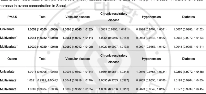
Table 6 estimated relative risk of mortality with increase in PM2.5 and ozone.
As the level of particulate level increased by 10 ㎍/㎥, the overall mortality rate in the single exposure model, increased by 1.0059 (95% CI 1.0050-1.0068, p<0.05), in the multiple exposure model adjusted
meterological factors, increased by 1.0041 (95% CI 1.0032-1.0050, p<0.05), and in the multiple exposure model, adjusting for ozone level, increased by 1.0039 (95% CI 1.0029-1.0048, p<0.05), and mortality due to vascular disease by 1.0060 (95% CI 1.0012-1.0108, p<0.05) times higher risk of mortality. As the level of ozone level, the mortality rate increased by 10 ppb, increased by 1.0280 (95% CI 1.0072-1.0488, p<0.05) times higher risk of mortality due to diabetes and increased by 1.0015 due to overall disease with statistically insignificant in the single exposure model, and increased 1.0021 (95% CI 0.9999-1.0044, p<0.10) in the multiple exposure model adjusted meterological factors, and in the multiple exposure model, adjusting for particulate matters, ozone was associated with 1.0007 times higher risk of overall mortality, however it was not statistically significant.
36
Table 6. Estimated relative risk (95% intervals) in daily disease-specific mortality per 10-μg/m3 increase in PM2.5 and 10 ppb
increase in ozone concentration in Seoul
PM2.5 Total Vascular disease Chronic respiratory
disease Hypertension Diabetes
Univariate 1.0059 (1.0050, 1.0068) 1.0088 (1.0045, 1.0132) 1.0089 (0.9996, 1.0181)§ 0.9928 (0.9794, 1.0061) 1.0067 (0.9983, 1.0152)
Multivariate* 1.0041 (1.0032, 1.0050) 1.0064 (1.0017, 1.0111) 1.0054 (0.9955, 1.0153) 0.9983 (0.9843, 1.0122) 1.0062 (0.9972, 1.0153)
Multivariate† 1.0039 (1.0029, 1.0048) 1.0060 (1.0012, 1.0108) 1.0029 (0.9927, 1.0132) 0.9997 (0.9853, 1.0142) 1.0048 (0.9955, 1.0141)
Ozone Total Vascular disease Chronic respiratory
disease Hypertension Diabetes
Univariate 1.0015 (0.9995, 1.0035) 1.0003 (0.9893, 1.0114) 1.0104 (0.9861, 1.0348) 1.0049 (0.9765, 1.0334) 1.0280 (1.0072, 1.0488)
Multivariate* 1.0021 (0.9999, 1.0044)§ 1.0044 (0.9919, 1.0170) 1.0055 (0.9783, 1.0327) 0.9869 (0.9550, 1.0188) 1.0199 (0.9964, 1.0435)
Multivariate‡ 1.0007 (0.9984, 1.0030) 1.0009 (0.9882, 1.0135) 1.0039 (0.9766, 1.0313) 0.9873 (0.9549, 1.0197) 1.0177 (0.9939, 1.0415)
*Estimates were generated using over-dispersed generalized linear models and polynomial distributed lag model for cumulative exposures over the same day and lag days, adjusted for calendar day {natural smooth function with 4*12 degrees of freedom (df)}, day of the week, temperature (lag 0, natural smooth function, 3 df), pressure (lag=0), humidity (lag 0). †Estimates were generated using multivariate model* and ozone (lag 0, natural smooth function, 3 df).
‡Estimates were generated using multivariate model* and PM2.5 (lag 0, natural smooth function, 3 df). §p-Value were less than 0.10.
37
4. Analysis of association in period specific outcome
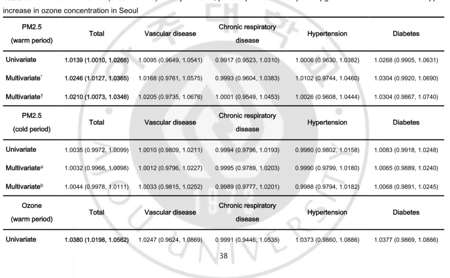
Table 7 estimated relative risk of period specific ER visit with increase in PM2.5 and ozone.
Considering the warm and cold period separately, with ozone as the main exposure factor, increase in the overall disease rate 1.0380 (95% CI 1.0198-1.0562, p<0.05) in the single exposure model, and in the overall disease rate 1.0323 (95% CI 1.0135-1.0511, p<0.05) in the multiple exposure model adjusted meterological factors were significant in the warm-period. However, in all disease types with ozone as main exposure factor, there were no significant results in the cold-period. In terms of PM2.5, increase in overall disease rate, 1.0139 times in the single exposure model, 1.0246 times in the multiple exposure model, and 1.0210 times higher in the multiple exposure model adjusting for ozone during the warm-period. However, during the cold-period, there were no significant results with PM2.5 as the main exposure factor.
38
Table 7. Estimated relative risk (95% intervals) in daily disease-, period-specific ER visit per 10-μg/m3 increase in PM2.5 and 10 ppb
increase in ozone concentration in Seoul
PM2.5
(warm period) Total Vascular disease
Chronic respiratory
disease Hypertension Diabetes
Univariate 1.0139 (1.0010, 1.0268) 1.0095 (0.9649, 1.0541) 0.9917 (0.9523, 1.0310) 1.0006 (0.9630, 1.0382) 1.0268 (0.9905, 1.0631)
Multivariate* 1.0246 (1.0127, 1.0365) 1.0168 (0.9761, 1.0575) 0.9993 (0.9604, 1.0383) 1.0102 (0.9744, 1.0460) 1.0304 (0.9920, 1.0690)
Multivariate† 1.0210 (1.0073, 1.0346) 1.0205 (0.9735, 1.0676) 1.0001 (0.9549, 1.0453) 1.0026 (0.9608, 1.0444) 1.0304 (0.9867, 1.0740)
PM2.5
(cold period) Total Vascular disease
Chronic respiratory
disease Hypertension Diabetes
Univariate 1.0035 (0.9972, 1.0099) 1.0010 (0.9809, 1.0211) 0.9994 (0.9796, 1.0193) 0.9980 (0.9802, 1.0158) 1.0083 (0.9918, 1.0248)
Multivariatea 1.0032 (0.9966, 1.0098) 1.0012 (0.9796, 1.0227) 0.9995 (0.9789, 1.0203) 0.9990 (0.9799, 1.0180) 1.0065 (0.9889, 1.0240)
Multivariateb 1.0044 (0.9978, 1.0111) 1.0033 (0.9815, 1.0252) 0.9989 (0.9777, 1.0201) 0.9988 (0.9794, 1.0182) 1.0068 (0.9891, 1.0245)
Ozone
(warm period) Total Vascular disease
Chronic respiratory
disease Hypertension Diabetes
39
Multivariate* 1.0323 (1.0135, 1.0511) 1.0102 (0.9477, 1.0726) 0.9986 (0.9389, 1.0583) 1.0336 (0.9789, 1.0883) 1.0277 (0.9664, 1.0889)
Multivariate‡ 1.0173 (0.9954, 1.0392) 1.0017 (0.9280, 1.0753) 1.0021 (0.9316, 1.0725) 1.0352 (0.9703, 1.1001) 0.9974 (0.9268, 1.0681)
Ozone
(cold period) Total Vascular disease
Chronic respiratory
disease Hypertension Diabetes
Univariate 1.0128 (0.9960, 1.0297) 1.0210 (0.9696, 1.0725) 1.0096 (0.9581, 1.0610) 1.0287 (0.9837, 1.0737) 0.9348 (0.8851, 0.9845)
Multivariate* 1.0033 (0.9853, 1.0215) 1.0158 (0.9593, 1.0722) 1.0008 (0.9460, 1.0556) 1.0251 (0.9757, 1.0744) 0.9304 (0.8755, 0.9852)
Multivariate‡ 1.0043 (0.9860, 1.0225) 1.0180 (0.9609, 1.0752) 1.0077 (0.9523, 1.0631) 1.0255 (0.9755, 1.0755) 0.9329 (0.8775, 0.9882)
*Estimates were generated using over-dispersed generalized linear models and polynomial distributed lag model for cumulative exposures over the same day and lag days, adjusted for calendar day {natural smooth function with 4*12 degrees of freedom (df)}, day of the week, temperature (lag 0, natural smooth function, 3 df), pressure (lag=0), humidity (lag 0). †Estimates were generated using multivariate model* and ozone (lag 0, natural smooth function, 3 df).
‡Estimates were generated using multivariate model* and PM2.5 (lag 0, natural smooth function, 3 df). §p-Value were less than 0.10.
40
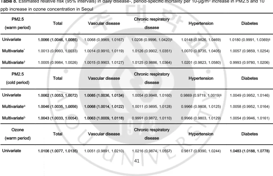
Table 8 estimated relative risk of period specific mortality with increase in PM2.5 and ozone.
Considering the warm and cold period separately, in the single and multiple exposure model, with ozone as the main exposure factor, increase in the overall mortality rate 1.0106 (95% CI 1.0077-1.0135, p<0.05) in the single exposure model, 1.0031 (95% CI 0.9998-1.0063, p<0.10) in the multi exposure model adjusted meterological factors, and mortality due to diabetes 1.0483 (95% CI 1.0188-1.0778, p<0.05) in the single exposure model, 1.0299 (95% CI 0.9954-1.0644, p<0.10) in the multi exposure model adjusted meterological factors were significant in the warm-period. Moreover, in the multiple exposure model, adjusting for PM2.5, the overall mortality rate increased by 1.0025, with statistically insignificant, due to ozone in the cold-period. In terms of PM2.5, overall mortality and due to vascular disease increased in all the models (overall mortality: 1.0062 times in the single model, 1.0046 in the multiple model adjusting for meterological factors, 1.0043 in the multiple model adjusting for ozone; vascular mortality: 1.0085 in the single model, 1.0068 in the multiple model adjusted meterological factors, 1.0063 in the multiple model adjusted for ozone, all p<0.05), during the cold-period. Also, during the warm-period, the overall mortality increased by 1.0066 times (95% CI 1.0046-1.0085, p<0.05) and due to diabetes, 1.0180 times (95% CI 0.9991-1.0369, p<0.10), and due to chronic pulmonary disease 1.0208 (95% CI 0.9996-1.0420, p<0.10) in the single exposure model.
41
Table 8. Estimated relative risk (95% intervals) in daily disease-, period-specific mortality per 10-μg/m3 increase in PM2.5 and 10
ppb increase in ozone concentration in Seoul
PM2.5
(warm period) Total Vascular disease
Chronic respiratory
disease Hypertension Diabetes
Univariate 1.0066 (1.0046, 1.0085) 1.0068 (0.9969, 1.0167) 1.0208 (0.9996, 1.0420)§ 1.0148 (0.9826, 1.0469) 1.0180 (0.9991, 1.0369)§
Multivariate* 1.0013 (0.9993, 1.0033) 1.0014 (0.9910, 1.0119) 1.0126 (0.9902, 1.0351) 1.0070 (0.9735, 1.0405) 1.0057 (0.9859, 1.0254)
Multivariate† 1.0005 (0.9984, 1.0026) 1.0015 (0.9903, 1.0127) 1.0125 (0.9886, 1.0364) 1.0201 (0.9823, 1.0580) 0.9993 (0.9780, 1.0206)
PM2.5
(cold period) Total Vascular disease
Chronic respiratory
disease Hypertension Diabetes
Univariate 1.0062 (1.0053, 1.0072) 1.0085 (1.0036, 1.0134) 1.0054 (0.9948, 1.0160) 0.9869 (0.9719, 1.0019)§ 1.0049 (0.9952, 1.0146)
Multivariatea 1.0046 (1.0035, 1.0056) 1.0068 (1.0014, 1.0122) 1.0011 (0.9895, 1.0128) 0.9966 (0.9808, 1.0125) 1.0058 (0.9952, 1.0164)
Multivariateb 1.0043 (1.0033, 1.0054) 1.0063 (1.0009, 1.0118) 0.9991 (0.9872, 1.0110) 0.9966 (0.9803, 1.0129) 1.0054 (0.9946, 1.0161)
Ozone
(warm period) Total Vascular disease
Chronic respiratory
disease Hypertension Diabetes
42
Multivariate* 1.0031 (0.9998, 1.0063)§ 1.0006 (0.9820, 1.0191) 1.0056 (0.9658, 1.0454) 0.9739 (0.9244, 1.0234) 1.0299 (0.9954, 1.0644)§
Multivariate‡ 1.0022 (0.9986, 1.0057) 0.9936 (0.9735, 1.0138) 1.0027 (0.9597, 1.0457) 0.9541 (0.8971, 1.0110) 1.0260 (0.9884, 1.0636)
Ozone
(cold period) Total Vascular disease
Chronic respiratory
disease Hypertension Diabetes
Univariate 0.9952 (0.9922, 0.9983) 0.9937 (0.9772, 1.0103) 0.9932 (0.9561, 1.0303) 1.0307 (0.9881, 1.0733) 1.0112 (0.9801, 1.0424)
Multivariate* 1.0006 (0.9971, 1.0041) 1.0030 (0.9839, 1.0223) 1.0045 (0.9618, 1.0472) 0.9905 (0.9416, 1.0394) 1.0055 (0.9693, 1.0417)
Multivariate‡ 1.0025 (0.9990, 1.0061) 1.0054 (0.9859, 1.0249) 1.0046 (0.9611, 1.0481) 0.9971 (0.9475, 1.0468) 1.0082 (0.9713, 1.0450)
*Estimates were generated using over-dispersed generalized linear models and polynomial distributed lag model for cumulative exposures over the same day and lag days, adjusted for calendar day {natural smooth function with 4*12 degrees of freedom (df)}, day of the week, temperature (lag 0, natural smooth function, 3 df), pressure (lag=0), humidity (lag 0). †Estimates were generated using multivariate model* and ozone (lag 0, natural smooth function, 3 df).
‡Estimates were generated using multivariate model* and PM2.5 (lag 0, natural smooth function, 3 df). §p-Value were less than 0.10.
43
5. Analysis of association according to lag day
Table 9 and Figure 3 estimated relative risk of ER visit with increase in PM2.5 and ozone according to lag days.
The relative risk of ER visit due to increase in PM2.5 level in the single exposure model was 1.0062 (95% CI 1.0006-1.0119, p<0.05) on the day of visit, 1.0058 (95% CI 1.0002-1.0115, p<0.05) one day after visit. The results of the lag effect in multiple exposure model adjusting for meterological factors are as follows: Lag 0 (day of visit): 1.0074, 95% CI 1.0015-1.0133; Lag 1: 1.0066, 95% CI 1.0008-1.0125; Lag 2: 1.0059, 95% CI 0.9999-1.0117; Lag 3: 1.0051, 95% CI 0.9992-1.0109; p<0.05, except Lag 2 (p<0.10) and Lag 3 (p<0.10). In the model with ozone as the exposure factor, adjusting for meterological factors, the lag effect remained significant until three days after visit, and was bigger compared to the model considering PM2.5 as the main exposure factor: Lag 0 (day of visit): 1.0185, 95% CI 1.0048-1.0321; Lag 1: 1.0166, 95% CI 1.0032-1.0300; Lag 2: 1.0150, 95% CI 1.0018-1.0281; Lag 3: 1.0136, 95% CI 1.0005-1.0266; all p<0.05). Lastly, in the multiple exposure model of ozone including PM2.5, the result was significant until one day after visit: Lag 0 (day of visit): 1.0162, 95% CI 1.0023-1.0300; Lag 1: 1.0143, 95% CI 1.0007-1.0278; all p<0.05).
44
Table 9. Estimated relative risk (95% interval) in daily ER visit per 10-μg/m3 increase in PM2.5 and 10 ppb increase in ozone
concentrations in Seoul, according to lag days.
PM2.5 Lag 0 Lag 1 Lag 2 Lag 3 Lag 4 Lag 5
Univariate 1.0062 (1.0006, 1.0119) 1.0058 (1.0002, 1.0115) 1.0055 (0.9998, 1.0111)§ 1.0051 (0.9994, 1.0107)§ 1.0046 (0.9990, 1.0103) 1.0044 (0.9987, 1.0101) Multivariate* 1.0074 (1.0015, 1.0133) 1.0066 (1.0008, 1.0125) 1.0059 (0.9999, 1.0117)§ 1.0051 (0.9992, 1.0109)§ 1.0043 (0.9985, 1.0102) 1.0038 (0.9980, 1.0096) Multivariate† 1.0057 (0.9996, 1.0118)§ 1.0049 (0.9989, 1.0110) 1.0042 (0.9982, 1.0102) 1.0036 (0.9976, 1.0095) 1.0029 (0.9970, 1.0089) 1.0025 (0.9966, 1.0084)
Ozone Lag 0 Lag 1 Lag 2 Lag 3 Lag 4 Lag 5
Univariate 1.0225 (1.0102, 1.0349) 1.0203 (1.0080, 1.0326) 1.0181 (1.0059, 1.0304) 1.0161 (1.0038, 1.0283) 1.0140 (1.0018, 1.0263) 1.0129 (1.0006, 1.0251) Multivariate* 1.0185 (1.0048, 1.0321) 1.0166 (1.0032, 1.0300) 1.0150 (1.0018, 1.0281) 1.0136 (1.0005, 1.0266) 1.0122 (0.9993, 1.0251)§ 1.0120 (0.9991, 1.0248)§ Multivariate‡ 1.0162 (1.0023, 1.0300) 1.0143 (1.0007, 1.0278) 1.0126 (0.9993, 1.0259)§ 1.0111 (0.9980, 1.0243)§ 1.0097 (0.9967, 1.0227) 1.0094 (0.9965, 1.0224)
45
*Estimates were generated using over-dispersed generalized linear models and polynomial distributed lag model for cumulative exposures over the same day and lag days, adjusted for calendar day {natural smooth function with 4*12 degrees of freedom (df)], day of the week, temperature (lag 0, natural smooth function, 3 df), pressure (lag=0), humidity (lag 0). †Estimates were generated using multivariate model* and ozone (lag 0, natural smooth function, 3 df).
‡Estimates were generated using multivariate model* and PM2.5 (lag 0, natural smooth function, 3 df). §p-Value were less than 0.10.
46
Figure 3. Estimated relative risk (95% interval) in daily ER visit per 10-μg/m3 increase in
PM2.5 and 10 ppb increase in ozone concentrations in Seoul, according to lag days (0~5).
Estimates were generated using over-dispersed generalized linear models and polynomial distributed lag model for cumulative exposures over the same day and lag days, adjusted for calendar day {natural smooth function with 4*12 degrees of freedom (df)}, day of the week, temperature (lag 0, natural smooth function, 3 df), pressure (lag=0), humidity (lag 0) and month.
47
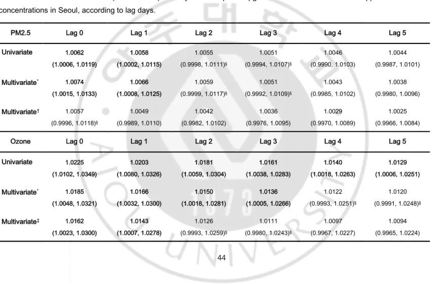
Table 10 and Figure 4 estimated relative risk of mortality with increase in PM2.5 and ozone according to lag days.
The relative risk of mortality due to increase in PM2.5 level in the single exposure model was 1.0059 (95% CI 1.0050-1.0068, p<0.05) on the day of death, 1.0057 (95% CI 1.0048-1.0065, p<0.05) one day after death. The results of the lag effect in the multivariate model adjusting for ozone are as follows: Lag 0 (day of death): 1.0039, 95% CI 1.0029-1.0148; Lag 1: 1.0037, 95% CI 1.0028-1.0046; Lag 2: 1.0035, 95% CI 1.0026-1.0044; Lag 3: 1.0034, 95% CI 1.0025-1.0043; Lag 4: 1.0032, 95% CI 1.0023-1.0042; Lag 5: 1.0032, 95% CI 1.0023-1.0040, all p<0.05). In the model with ozone as the exposure factor, adjusting for meterological factors, the lag effect remained little significant on the day of death, and was smaller compared to the model considering PM2.5 as the main exposure factor: Lag 0 (day of death): 1.0021, 95% CI 0.9999-1.0044, p<0.10). Lastly, in the multiple exposure model of ozone including PM2.5, the result were no significant in all lag days.
48
Table 10. Estimated relative risk (95% interval) in daily mortality per 10-μg/m3 increase in PM2.5 and 10 ppb increase in ozone
concentrations in Seoul, according to lag days.
PM2.5 Lag 0 Lag 1 Lag 2 Lag 3 Lag 4 Lag 5
Univariate 1.0059 (1.0050, 1.0068) 1.0057 (1.0048, 1.0065) 1.0055 (1.0046, 1.0063) 1.0052 (1.0044, 1.0061) 1.0050 (1.0042, 1.0059) 1.0048 (1.0039, 1.0057) Multivariatea 1.0041 (1.0032, 1.0050) 1.0039 (1.0030, 1.0048) 1.0037 (1.0028, 1.0046) 1.0036 (1.0027, 1.0045) 1.0034 (1.0025, 1.0043) 1.0033 (1.0024, 1.0042) Multivariateb 1.0039 (1.0029, 1.0048) 1.0037 (1.0028, 1.0046) 1.0035 (1.0026, 1.0044) 1.0034 (1.0025, 1.0043) 1.0032 (1.0023, 1.0042) 1.0032 (1.0023, 1.0040)
Ozone Lag 0 Lag 1 Lag 2 Lag 3 Lag 4 Lag 5
Univariate 1.0015 (0.9995, 1.0035) 1.0005 (0.9986, 1.0026) 0.9996 (0.9976, 1.0016) 0.9987 (0.9976, 1.0007) 0.9977 (0.9957, 0.9998) 0.9968 (0.9948, 0.9988) Multivariatea 1.0021 (0.9999, 1.0044)§ 1.0014 (0.9992, 1.0036) 1.0007 (0.9985, 1.0029) 1.0001 (0.9979, 1.0022) 0.9994 (0.9973, 1.0016) 0.9988 (0.9966, 1.0009) Multivariatec 1.0007 (0.9984, 1.0030) 1.0000 (0.9978, 1.0022) 0.9994 (0.9972, 1.0016) 0.9988 (0.9966, 1.0010) 0.9982 (0.9960, 1.0003) 0.9976 (0.9954, 0.9997)
49
aEstimates were generated using over-dispersed generalized linear models and polynomial distributed lag model for cumulative exposures over the same day and lag days, adjusted for calendar day {natural smooth function with 4*12 degrees of freedom (df)}, day of the week, temperature (lag 0, natural smooth function, 3 df), pressure (lag=0), and humidity (lag 0). bEstimates were generated using multivariate model* and ozone (lag 0, natural smooth function, 3 df).
cEstimates were generated using multivariate model* and PM2.5 (lag 0, natural smooth function, 3 df). dp-Value were less than 0.10.