1. INTRODUCTION
As the personal computer in old times, the price of robot is gradually decreasing and many scientists said that the time will comes soon that one family have one robot. The fact that the government selected the intelligent robot one of the 10 next generation of enterprise is speaking well the importance of robot industry. Among them, the research about humanoid robot has been processed actively. The humanoid robot has large value of practical use in the point of view that it has same task region with human. Japan, which is leading country in robot, advanced the technique more in humanoid robot like what ASIMO of HONDA and SDR of SONY. Currently, the development of the biped walking robot has been preceded actively, but truly do not reach the Japan yet.
We said that the biped walking robot is the robot which walks with 2 legs like human. In order to imitate the human's motion, generally each leg got 6 degree of freedoms and controlled by microprocessor or microcontroller.
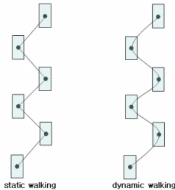
Figure 1. The path of center of gravity
The control algorithm is divided into static walking and dynamic walking. Each part of the path of Static walking has straight line as the motion pattern is acted sequentially, and the dynamic walking has curved path as the motion pattern is acted continuously. These control algorithms are various according to various forms of sensor interfaces and various theories.
In this paper, we propose to apply the principle of inverted pendulum to implement stable walking. The robot's motions are implemented with mechanical analysis except the notion of force, and implement more stable walking with the principle of inverted pendulum.
2. THE COMPOSITION OF ENTIRE SYSTEM
AND OVERVIEW OF MOTION CONTROL
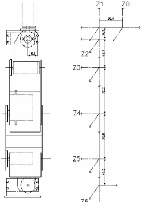
Figure 2. The entire system
The robot system is composed with the wireless modem which is connected with the laptop computer, robot's body and the controller which is loaded in the body of the robot. The
Development of a Biped Walking Robot
Yong-Sung Kim
*, Chang-Jun Seo
*** Department of Electronics Engineering, Kyungpook National University, Daegu 702-701, Korea
(Tel : +82-53-940-8853 E-mail: [email protected])
** Department of Electronics Engineering, Inje University, Kimhae 621-749 , Korea
(Tel : +82-55-320-3438 E-mail:
[email protected]
)Abstract: In this paper, we introduce biped walking robot which can static walking with 22 degree-of-freedoms. The developed biped walking robot is 480mm tall and 2500g, and 22 RC servo motors are used to actuate. Before made an active algorithm, we generated the motions of robot with the motion simulator which developed using by C language. The two dimension simulator is Based on the inverse kinematics and D-H transform. The simulator implements various motions as inputted the ankle's trajectory. Also we developed a simulator which is applied the principle of inverted pendulum to acquires the center of gravity. As we use this simulator, we can get the best appropriate angle of ankle and pelvis when the robot lifts up its one side leg during the working. We implement the walking motions which is based on the data(angle) getting from both of simulators. The robot can be controlled by text shaped command through RF signal of wireless modem which connected with laptop computer by serial cable.
robot is controlled by text shaped command through RF signal of wireless modem which connected with laptop computer by serial cable. The robot conducts the pre-programmed action according to the received command.
The walking of the robot is implemented repeating the sequence like stretching right leg, moving center of gravity to the right and then stretching left leg, moving center of gravity to the left. The action of stepping forward is implemented by applying the angles that getting from 2 dimension motion simulator. And the result(angles) of simulation about one leg can apply to the opposite side leg. Because the sign of opposite side leg's angle is contrast. Thus we simulated about one side leg only. Also we developed a simulator which is applied the principle of inverted pendulum to acquire the center of gravity. The simulator about center of gravity acquires the best angle of ankle and pelvis when the robot moves the center of gravity to left and right side, and we applied the acquired angle to the robot control.
3. THE PROCESS OF DEVELOPMENT AND
DESIGN
3.1 Setting up the coordinate system of each joint.
At first, we selected the degree of freedoms of each joint, and selected the suitable sequence of Yaw, Roll, and Pitch to combine organically. Then, we defined the center of each pelvis to a reference coordinate system, and the Z axis of each coordinate system of joints was set to the axis of rotation. The coordinate system of developed robot is set through the D-H representation and the content is as follows.
(DH 1) The axis X1 is orthogonal to Z0 (DH 2) Axis X1 meets the axis Z0
Figure 3. The coordinate systems of leg
Figure 4. Designed the body using Auto CAD
Table 1. D-H parameters of each joints
Joint ai
α
i diθ
i 2(Yaw) 0 -90 d2(-)θ
2 3(Roll) a3 90 0θ
3 4(Pitch) a4 0 0θ
4 5(Pitch) a5 0 0θ
5 6(Pitch) a6 0 0θ
6 7(Roll) a7 -90 0θ
7The meaning of D-H parameters are as follows.
i
a: The distance between Zi-1 and Zi (It exist when the two axis Z does not meet each other, It's Determined by the axis Xi)
i
α
: The angle between Zi-1 and Zi (It's Determined at the plane that is orthogonal to the axis Xi)i
d : The distance between Oi-1, the origin of coordinate system i-1, and the Intersection of Xi and Zi-1.
i
θ
: The angle between axis Xi-1 and axis Xi (It's Determined at the plane that is orthogonal to the axis Zi-1)The reason why the parameter of the joint 1 does not exist in table 1 is that we set the 1
0
R to Tans(d1) Rot(z,-90).
When we set the center of each pelvis to the reference coordinate system, the transformation matrix of each link is as follows. 1 0 0 1 0 0 1 0 0 0 0 1 0 0 0 0 1 a R − − =
2 2 2 2 2 1 2 0 0 0 0 0 1 0 0 0 0 1 C S S C R d θ θ θ θ − = − − 3 3 3 3 3 3 3 3 3 2 0 0 0 1 0 0 0 0 0 1 C S a C S C a S R θ θ θ θ θ θ − = 4 4 4 4 4 4 4 4 4 3 0 0 0 1 1 0 0 0 0 1 C S a C S C a S R θ θ θ θ θ θ − = 5 5 5 5 5 5 5 5 5 4 0 0 0 0 1 0 0 0 0 1 C S a C S C a S R θ θ θ θ θ θ − = 6 6 6 6 6 6 6 6 6 5 0 0 0 0 1 0 0 0 0 1 C S a C S C a S R θ θ θ θ θ θ − = 7 6 7 7 7 7 7 7 7 6 0 0 0 1 1 0 0 0 0 1 C S a C S C a S R θ θ θ θ θ θ − = − The i i
R−1 means the matrix which express the ith joint’s
coordinate system regarding the i-1th joint’s coordinate system. 1 1 0 0
T
=
R
2 1 2 0 0 1T
=
R R
M
6 1 2 3 4 5 6 0 0 1 2 3 4 5T
=
R R R R R R
7 1 2 3 4 5 6 7 0 0 1 2 3 4 5 6T
=
R R R R R R R
(1)
By getting the 1 0 T ~ 7 6T , we can express and analyze each joint's coordinates with respect to the reference coordinate system.
3.2 Generating the motion with inverse kinematics
.
The forward kinematics is a study to get the coordinate of end effector, on the other hand the inverse kinematics is to get the angle of joint which make the end effector coincide with thearbitrary position we want. Inverse kinematics has various solutions unlike forward kinematics. But we can get the only one solution as we give the range to each axis of rotation.
There are various methods of inverse kinematics, but most of the methods are very difficult to use. So we use the iterative method in programming. Namely, the method is to find the most approximated solution with changing the each joint's angle one by one inside the range. The developed robot act static walking as repeating the following sequence, stretching right leg, moving center of gravity to the right, and then stretching left leg, moving center of gravity to the left. Thus, when the one side leg steps on, the stepping leg's angle of pelvis and ankle and the opposite side leg's angles of each joint do not change. That means we can reduce the variable when we think about the varying angle only.
Consequently, there remain only three variables to simulate, the
θ
4,θ
5andθ
6 corresponding to pitch of stepping leg. If we assume that the sole is always parallel to surface,θ
6can expressed by combination of θ4 andθ
5. Namely, we can get the approximated solution as changing theθ
4 andθ
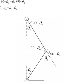
5 only. Hence, we can get (2) from figure 5.90+
θ
6=θ
5+90-θ
4∴
θ
6=θ
5-θ
4 (2)Figure 5. Explaining the elimination of
θ
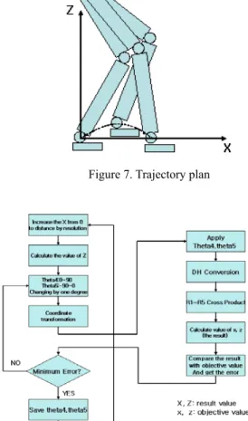
6The last process is trajectory plan. The trajectory was set simply to second order function, and the formula of trajectory is expressed as follow.
(
)
2(
)
2 peak y x x distance distance = − ⋅ − (3)Figure 6. Setting of trajectory
We should execute repeatedly the (1) when trajectory was set to the tip of toes. But we can ignore the 6
5
R , 7 6
R when we set trajectory about the ankle. Although the 6
5
R and 7 6
R are ignored, the result is same. Because, we assume that the sole is parallel to the surface.
We designed the simulator according to the settings and assumptions. Also we saved the result of coordinate of each joints, then display sequentially whether the motion acting smoothly.
Figure 7. Trajectory plan
Figure 8. The algorithm of simulation
3.3 Applying and analyzing the principle of inverted pendulum for stabilization of robot while working
.
The most important thing when implement the robot’s walking is do not fall down, namely implement the stable walking. The moment which the robot comes to be most unstable is the moment which the robot lifts up its one side leg. In this paper, we try to apply the principle of inverted pendulum instead of try&error method for stable walking.
As simply each part of the body to one point mass and ignore the each of link’s weight, we can assume the each masses to inverted pendulum which connected to the ankle with length ℓ when the roll of ankle act to axis of rotation. And as we set simulation environment to 2 dimension coordinate whose origin is roll of ankle corresponding to axis of rotation, the center point of each masses are expressed to the coordinate which is about axis x and y. When each of point masses are defined, we can get the straight line ℓ which connected to the origin and angle
θ
between ℓ and axis y. If we assume the gravity acceleration g is regular, then the torque will be the function of m, ℓ andθ
. When we put the m to the constant, the torque can be calculated by only the point mass’s coordinate.As you see at figure 10, we can suppose that the position is the balanced position when the sum of torque of left and right side became equal. Namely, when disregarding inertia, we can assume that the projection point of center of gravity to axis x is in the origin.
Figure 9. The torque of each point mass
In the walking process, the robot increase the angle of ankle and pelvis according to the roll to
θ
before it stretch its leg, at this time, we should find the optimized angle ofθ
to do not fall down Statically. When we assume the optimized angle isθ
s, theθ
which holds (4) is theθ
s makes the robot to be the most stabilized.(Letθ
s to ‘balanced angle’)1 i 1 i n n R L i i
T
T
= ==
∑
∑
(4)
According to the condition until now, we developed the simulator about center of gravity which can determine thevariance of left and right torques, and which can find the angle of roll of the ankle and pelvis to make the robot to be the most stabilized. The developed simulator about center of gravity does not use the transformation matrix for more rapid calculation. Transformation matrix is based on the 3 dimension. Because we do not tread the side of the robot, we set the coordinate of robot to 2 dimensions whose origin is roll of ankle corresponding to axis of rotation. And the process of calculating the coordinate of each point masses is explained at figure 11, 12 and 13.
Figure 11. Deriving the coordinate of right leg
Figure 12. Deriving the coordinate of body
Figure 13. Deriving the coordinate of left leg From the figure 11, 12 and 13, we can see that the coordinate of masses of right leg is determined by
θ
1, and the bodydetermined by
θ
1 andθ
2, and the left leg is determined by1
θ
,θ
2 andθ
3.Lastly, to find the torque of the point masses, there needs some process of linearization of the formula about torque T. The torque of inverted pendulum is as follow.
θ
sin
mgl
T
=
(5)Figure 14. Torque of inverted pendulum.
The (5) can be linearization with using the term of first order of Taylor Series. If we set the m, g, ℓ to constant and the torque is only function of
θ
, then, it can be expressed as follows.( )
( )
( ) (
)
( )
( )
(
)
0 ' 0 0 0 0 0 1! sin sin T T T d mgl mgl d θ θθ
θ
θ
θ θ
θ
θ
θ θ
θ
= = + − = + ⋅ − (6) The (6) be the Maclaurin Series When we setθ
0 to zero, and then we can get the formula as follows.) (
θ
T =mglsin(0)+mglcos(0)(θ
−0) =mglθ
T mglθ
∴ = (7) According to (7), we calculated the torque of left and right side, and we can find the angle of roll and pelvis, namelyθ
s, which makes the robot to be most stabilized.3.4 22 servo motor control which use microcontroller AVR
The actuator of developed robot is digital servo and it can be controlled by periodic duty signal. There needs some process to input duty signal to many servos in limited number of timers, like what generating time-divided signal of the timer.
We use ATmega128 which is one of the microcontroller AVR, and we do not explain concretely about it. We will explain the algorithm of motor control only. The microcontroller ATmega128 has 2 8bit timers and 6 16bit timers. Among them, we use one 8bit timer and two 16bit timers to actuate both legs(12 motors) and body(2 motors). And the both arms(8 motors) are actuated by one 16bit timer. Eventually, 22 motors are actuated by 4 timers among 8 timers. The servo motor can be controlled by periodic duty signal which is time-divided.
4. EXPERIMENT AND SIMULATION
Figure 15. Forward short
Figure 16. Forward long
Figure 17. Backward
Table 2. The result of motion simulation
Forward short Forward long backward
Time 4
θ
θ
5θ
4θ
5θ
4θ
5 t 30 -60 0 -44 30 -60 t+∆t 38 -72 12 -62 33 -72 t+2∆t 44 -79 22 -75 34 -79 t+3∆t 49 -83 31 -83 33 -83 t+4∆t 53 -85 38 -87 31 -85 t+5∆t 56 -85 44 -89 28 -85 t+6∆t 57 -82 49 -87 24 -82 t+7∆t 57 -78 52 -83 20 -77 t+8∆t 54 -69 53 -75 15 -70 t+9∆t 50 -58 50 -62 8 -59 t+10∆t 43 -42 43 -42 0 -44Figure 18. The result of center of gravity simulation The table 2 is result of the motion simulation, and we can get
s
θ
=14, the balanced angle, as the result of the simulation about center of gravity. But, there's some error when we apply the data of results to the robot. The biggest reasons are probably the mechanical freeplay and the backlash inside of motor. Especially, In the case of ankle and pelvis, the freeplay will be larger because of the excessive force, and then the walking is more unstable. We revised the mechanical freeplay with changing motor horn and strengthen the connection, also the backlash is revised by programming.5. CONSLUSION
In this paper, we introduced biped walking robot which can static walking with 22 degree-of-freedoms. The developed robot can forward and backward walking and left and right turning, and it controlled by text shaped command which transmitted by wireless modem that connected by laptop PC. The developed simulator of motion and center of gravity can apply to the different size robot. If the degree of freedoms and the sequence of Yaw-Roll-Pitch are same, the different size robot can be applied to the simulators with changing some parameters(m and ℓ), and advances the time of implementation of the motion.
We should proceed the research about the control algorithm using various sensor like FSR(Force Sensing Resistor) and slope sensor for real-time revising the attitude, and also proceed the development of simulator which integrates the motion and center of gravity.
REFERENCES
[1] Mark W.Spong, M. Vidyasagar, “Robot dynamics and control”, John Wiley & Sons, 1989
[2] Jang-Myeong Lee, jinyoung, “Introduction of Robotics”, 2003
[3] Young-Whui Sung, Su-young Lee, “The development of a miniature humanoid robot system”, The institute of control automation and systems engineers, 2001.5 [4] Young-Whui Sung, “A study on the inverse kinematics
for a biped robot”, The institute of control automation and systems engineers, 2003.12
[5] Duck-Yong Yoon, “AVR ATmega128 master”, Ohm, 2004