Chapter 8

(1)

The Complete Response of RL and RC Circuits

Seoul National University

Department of Electrical and Computer Engineering

Prof. SungJune Kim

(2)

Department of Electrical and Computer Engineering, SNU Prof. SungJune Kim

What is First Order Circuits?



Circuits that contain only one inductor or only one capacitor can be represented by a first-order differential equation. These circuits are called first-order circuits

(a) First, separate the energy storage element from the rest of the circuit.

(b) Next, replace the circuit connected to a capacitor by its Thevenin equivalent circuit, or replace the circuit connected to an inductor by its Norton equivalent

circuit. (because the voltage in capacitor circuit or the current in inductor circuit are to be continuous.)

(3)

Response of the First Order Circuits



Consider the first-order circuit shown in Figure 8.2-2

 The circuit is at steady state before the switch is closed

 The switch closes at time t=0.

 After the switch is closed, the capacitor voltage is

0 ),

1000 cos(

)

(t = B t + t <

v

φ

0 ),

cos(

) 0

( = B t =

v

φ

) 1000

cos(

)

(t = Ke⁻ ^/^τ + M t +

δ

v ^t

Transient response

Steady-state response

(8.2-3)

(4)

The responses are called:

 “transient part of the response”  transient response

 “steady-state part of the response”  steady state response

 The response, v(t), given by Eq. 8.2-3, is called the complete response

 In general, the complete response of a first-order circuit can be represented as the sum of two part, the natural response ( which is the transient response) and the forced response (which is the steady state response):

 Natural response: the general solution of the (homogeneous) differential equation representing the first-order circuit, when the input is zero.

 Forced response: a particular solution of the differential equation representing the circuit when there is non-zero input.

complete response= transient response+ steady state response

complete response= natural response+ forced response

(5)

The names



The natural response of a first-order circuit will be of the form

When t

₀

=0, then

The constant K in the natural response depends on the initial condition.

For example, the capacitor voltage at time t

₀

τ / ) 0

response (

natural = Ke⁻ ^t⁻^t

τ

response /

natural = Ke⁻^t

(6)

Special Inputs to the First Order Circuits



In this chapter, we will consider three cases.

In theses cases the input to the circuit after the disturbance will be (1) a constant

(2) an exponential

(3) a sinusoid

These three cases are special because the forced response will have the same form as the input.

o

s t V

v ( ) =

τ /

) 0

( ^t

s t V e

v = ⁻

) cos(

)

(t =V₀ ωt+θ v_s

(7)

Plans to find complete response



Here is our plan for finding the complete response of first-order circuits:

Step 1: Find the steady state (forced) response before the disturbance. Evaluate this response at time t=t₀ to obtain the initial condition of the energy storage

element. (X(0): where it comes from.)

Step 2: Find the steady state (forced) response after the disturbance. (X(∞): where it goes ultimately.)

Step 3: Add the transient (natural) response=Ke^-t/^τ to the steady state (forced)

response to get the complete response. Use the initial condition to evaluate the constant K.

(8)

The Response of a First-Order Circuit to a Constant Input

 In Figure 8.3-1a we find a first-order circuit.

 X(0)= (R3/(R1+R2+R3)*Vs is the initial Steady State response

 X(∞)= (R3/(R2+R3)*Vs is the final Steady State response.

 The transient response can be obtained using the Thevenin circuit shown in Fig.8.3-1b.

and

3

2 3

oc s

V R V

R R

= +

2 3

t

s

R R R

R R

= +

FIGURE 8.3-1

(9)

The Response of a First-Order Circuit to a Constant Input

 The capacitor current is given by

 Apply KVL to Figure 8.3-1b to get

 Therefore,

( ) d ( ) i t C v t

= dt

( ) ( )

(

( )

)

( )

oc t t

V R i t v t R C d v t v t

= + = dt +

( ) V_oc

d v t

+ = ^(8.3-1)

FIGURE 8.3-1

(10)

Repeat the same for the inductor circuit using Norton eq. circuit.

2 s sc

I V

= R ² ³

2 3

t

s

R R R

R R

= +

FIGURE 8.3-2

(11)

Solving the inductor circuit

 The inductor voltage is given by

 Apply KCL to Figure 8.3-1b to get

 Therefore,

( ) d ( ) v t L i t

= dt

( ) ( )

sc

t t

L d i t

v t dt

I i t i t

R R

= + = +

R R

d + =

FIGURE 8.3-2

(12)

Now coming to a general form of solution

 Equation 8.3-1 and 8.3-2 have the same form. That is ( ) ( )

d x t

x t K

dt ⁺ τ ⁼

 The parameter τ is called the time constant. We will solve this differential equation by separating the variables and integrating. Then we will use the solution of Eq. 8.3-3 to obtain solutions of Eqs. 8.3-1 and 8.3- 2

 We may rewrite Eq. (3) as

dx K x

dt

τ τ

= −

 Or, separating the variables,

dx dt

x k− τ ^{= −} τ

(8.3-3)

(13)

Second page--

 Forming the indefinite integral, we have 1

dx dt D

x−kτ ^{= −}τ ⁺

∫ ∫

 Solving for x gives

( ) ^t/

x t = Kτ + Ae⁻ ^τ

where A=e^D, which is determined from the initial condition, x(0).

where D is a constant of integration. Performing the integration, we have

ln( ) t

x Kτ D

− = − +τ

(14)

Here we go. Note the solution at the bottom of this page.

 To find A, let t=0. Then (0) 0 /

x = Kτ + Ae⁻ ^τ = Kτ + A

 Therefore, we obtain

( ) [ (0) ] ^t/

x t = Kτ + x − K eτ ⁻ ^τ or

(0)

A= x −Kτ

 Since

( ) lim ( )

x t x t Kτ

∞ = →∞ =

 This can be written as

( ) ( ) [ (0) ( )] ^t/

x t = ∞ +x x − ∞x e⁻ ^τ

(15)

The plot

 Figure 8.3-3 shows a plot of x(t) versus t.

 We can determine the values of (1) the slope of the plot at time t=0 (2) the initial value of x(t)

(3) the final value of x(t) from this plot.

FIGURE 8.3-3

A graphical technique for measuring the

(16)

Apply this to the capacitor circuit

 Next, we apply these results to the RC circuit in Figure 8.3-1. Comparing Eqs.

8.3-1 and 8.3-3, we see that

( ) ( ), _t , ^oc

t

x t v t R C and k V τ R C

= = =

 Making these substitutions in Eq. 8.3-4 gives

/( )

( ) _oc ( (0) _oc) ^{t R C}^t v t =V + v −V e⁻

 This is the steady-state or forced response. The sum of the natural and forced responses is the complete response;

complete reponse = v t( ), forced response =V_OC

/( )

natural reponse = ( (0)v −V_OC)e⁻^{t R C}^t

(17)

Apply this to the inductor circuit

 Next, compare Eqs. 8.3-2 and 8.3-3 to find the solution of the RL circuit in Figure 8.3-2. We see that

( ) ( ), , _SC

t t

L L

x t i t and K I

R R

τ

= = =

 Making these substitutions in Eq. 8.3-4 gives

( / )

( ) _SC ( (0) _SC) ^{R L t}^t i t = I + i − I e⁻

 Again, the complete response is the sum of the forced(steady-state) response and the transient(natural) response:

complete reponse = i t( ), forced response = I_SC

( / )

natural reponse = ( (0)i − I_SC)e⁻ ^{R L t}^t

(18)

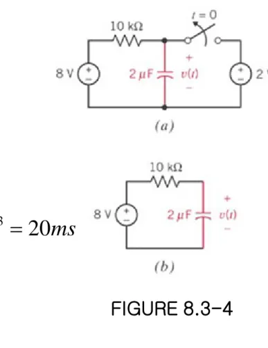
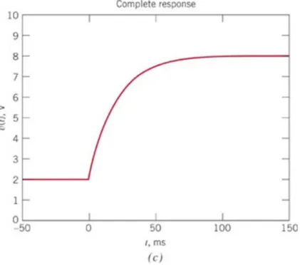
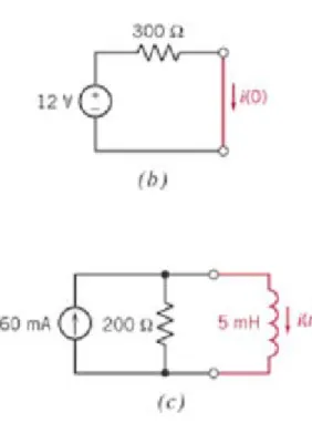
Example 8.3-1 First-Order Circuit with a Capacitor

 Find the capacitor voltage after the switch opens in the circuit shown in Figure 8.3-4a.

What is the value of the capacitor voltage 50ms after the switch opens?

(19)

Solution

10 8V

t OC

R = kΩ and V =

Initial condition

Figure 8.3-4b shows the circuit after the switch opens.

(0) 2V

v =

FIGURE 8.3-4

3 6 3

(10 10 )(2 10 ) 20 10 20

R C

t

ms

τ = = × ×

⁻

= ×

⁻

=

Time constant

Capacitor voltage

( ) 8 6

^t/ 20

V v t = − e

⁻

where t has units of ms.

(20)

Solution

To find the voltage 50ms after the switch opens, let t=50. Then

50 / 20

(50) 8 6 7.51V

v = − e

⁻

=

FIGURE 8.3-4 Figure 8.3-4c shows a plot of the capacitor voltage as a function of time

(21)

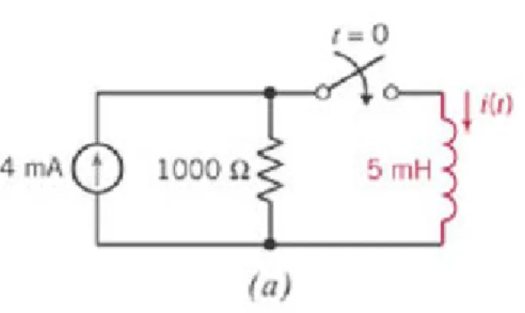
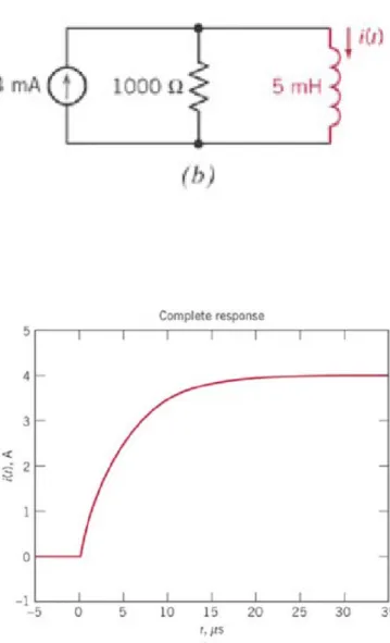
Example 8.3-2 First-Order Circuit with an Inductor



Find the inductor current after the switch closes in the circuit shown in

Figure 8.3-5a. How long will it take for the inductor current to reach 2mA?

FIGURE 8.3-4

(22)

Solution

3

5 10 6

5 10 5

t 1000

L s

τ

= R = ^× ⁻ = × ⁻ =

µ

( ) 4 4 ^t/ 5

i t = − e⁻ mA

1000 4

t SC

R = Ω and I = mA

Figure 8.3-5b shows the circuit after the switch closes.

Time constant

Inductor current

2 = −4 4e⁻^t/ 5mA

Find the time when the current reaches 2mA.

5 ln(2 4) 3.47 t = − × ⁻4 = µs

−

Figure8.3-5c shows a plot of the inductor current as a function of time

(23)

Example 8.3-3 First-Order Circuit

 The switch in Figure 8.3-6a has been open for a long time, and the circuit has

reached steady state before the switch closes at time t=0. Find the capacitor voltage for t≥0.

FIGURE 8.3-6

(24)

 Figure 8.3-6b shows the appropriate equivalent circuit while the switch is open.

Analyzing the circuit in Figure 8.3-6b using voltage division gives

Solution

3

3 3

60 10

(0) 12 7.2V

40 10 60 0

v ×

= =

× + ×1

 Figure 8.3-6c shows the appropriate equivalent circuit after the switch closes.

After the switch is closed

3

3 3

60 10

12 8V 30 10 60 0

v

OC

×

= =

× + ×1

3 3

3

3 3

30 10 60 10

20 10 20k Ω 30 10 60 0

R

t

= × × × = × =

× + ×1

(25)

 Consequently

where t has units of ms.

Solution

( ) 8 0.8

^t/ 40

V v t = − e

⁻

 The time constant is

3 6 3

(20 10 ) (2 10 ) 40 10 40ms R

t

C

τ = × = × × ×

⁻

= ×

⁻

=

(26)

 The switch in Figure 8.3-7a has been open for a long time, and the circuit has

reached steady state before the switch closes at time t=0. Find the inductor current for t≥0.

Example 8.3-4 First-Order Circuit

FIGURE 8.3-7

(27)

1. Figure 8.3-7b shows the appropriate equivalent circuit while the switch is open.

The initial inductor current can be calculated using Ohm’s law:

2. Figure 8.3-7c shows the appropriate equivalent circuit after the switch closes.

After the switch is closed

3. The time constant is

4. Consequently,

Solution

(0) 12 40mA i = 300 =

12 60mA and 200Ω

SC 200 t

I = = R =

( ) 60 20 ^t/ 25mA i t = − e⁻

3

5 10 6

25 10 25

t 200

L s

τ = R = ^× ⁻ = × ⁻ = µ

(28)



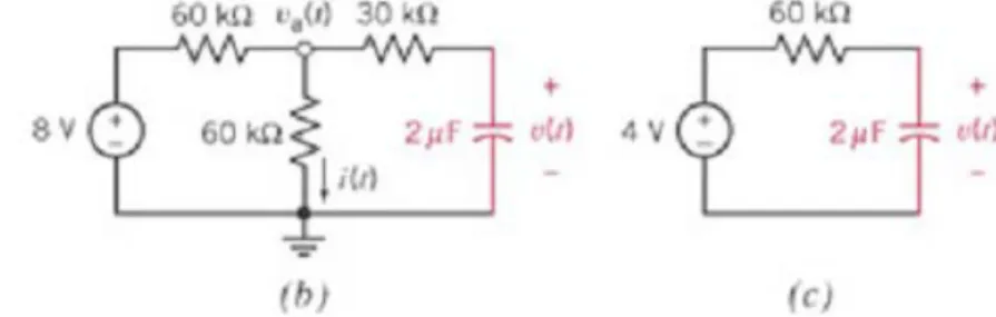
The circuit in Figure 8.3-8a is at steady state before the switch opens. Find the current i(t) for t>0.

Example 8.3-5 First-Order Circuit

FIGURE 8.3-8

(29)

1. We find the capacitor voltage. Before the switch opens, the capacitor voltage is equal to the voltage of the 2-volt source. The initial condition is

2. Figure 8.3-8b shows the circuit as it will be after the switch is opened.

The part of the circuit connected to the capacitor has been replaced by its Thévenin equivalent circuit in Figure 8.3-8c.

The parameters of the Thévenin equivalent circuit are

Solution

(0) 2V

v =

3

3 3

60 10

8 4V 60 10 60 0

vOC ×

= =

× + ×1

3 3

3 60 10 60 10 3

30 10 60 10 60kΩ

R × × ×

= × + = × =

(30)

therefore,

where t has units of ms

4. The node voltage, v_a(t) in Figure 8.3-8b

Solving for va(t), we get

5. Finally, we calculate I(t) using Ohm’s law:

Solution

3 6 3

(60 10 ) (2 10 ) 120 10 120ms Rt C

τ

= × = × × × ⁻ = × ⁻ =

3 3 3

( ) 8 ( ) ( ) ( )

60 10 60 10 30 10 0

a a a

v t − v t v t −v t

+ + =

× × ×

( ) 4 2 ^t/120V v t = − e⁻

/120

3 3 3

( ) 8 ( ) ( ) (4 2 ) 60 10 60 10 30 10 0

t

a a a

v t − v t v t − − e⁻

+ + =

× × ×

/120

8 2(4 2 ) /120

( ) 4 V

4

t

t a

v t e e

− −

+ −

= = −

/120

3 3

( ) 4

( ) 66.7 16.7

60 10 60 10

t a t

v t e

i t = = ⁻ ⁻ = − e⁻ µA

× ×

(31)

 Find the capacitor voltage after the switch opens in the circuit shown in Figure 8.3- 9a. What is the value of the capacitor voltage 50ms after the switch opens?

Example 8.3-6 First-Order Circuit with t

₀

≠0

FIGURE 8.3-9

(32)

1. The 2-volt voltage source forces the capacitor voltage to be 2 volts until the switch opens. Consequently,

2. In particular, the in initial condition is

3. Figure 8.3-8b shows the circuit after the switch opens. We see that

4. The time constant for this first-order circuit containing a capacitor is

5. Consequently, the voltage of the capacitor is given by

Solution

( ) 2V 0.05s

v t = for t ≤ (0.05) 2V

v =

10kΩ and 8V

t oc

R = V =

0.020s R Ct

τ = =

( 50) / 20

( ) 8 6 ^t V v t = − e^{− −}

(33)

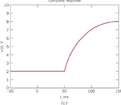
6. To find the voltage 50ms after the switch opens, let t=100ms. Then

7. Figure 8.3-9c shows a plot of the capacitor voltage as a function of time.

Solution

(100 50) / 20

(100) 8 6 =7.51V v = − e⁻ ⁻

(34)



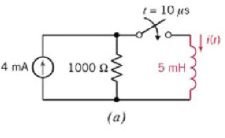
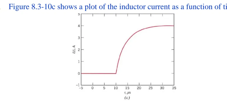
Find the inductor current after the switch closes in the circuit shown in

Figure 8.3-10a. How long will it take for the inductor current to reach 2mA?

Example 8.3-7 First-Order Circuit with t

₀

≠0

FIGURE 8.3-10

(35)

1. The inductor current will be 0A until the switch closes. There, the initial condition is

2. Figure 8.3-10b shows the circuit after the switch closes. We see that

3. The time constant for this first-order circuit containing an inductor is

4. Consequently, the current of the inductor is given by

Solution

(10 ) 0A i µ s =

1000Ω and 4mA

t SC

R = I =

3

5 10 6

5 10 5μs

t 1000 L

τ = R = ^× ⁻ = × ⁻ =

( 10) / 5

( ) 4 4 ^t mA i t = − e^{− −}

(36)

6. To find the time when the current reaches 2mA, substitute i(t)=2mA. Then

Solving for t gives

7. Figure 8.3-10c shows a plot of the inductor current as a function of time.

Solution

( 10) / 5

2 = −4 4e^{− −}^t mA

5 ln 2 4 10 13.47μs t = − ×  −−4 + =

(37)

 Figure 8.3-11a shows a plot of the voltage across the inductor in Figure 8.3-11b.

a. Determine the equation that represents the inductor voltage as a function of time.

b. Determine the value of the resistance R.

c. Determine the equation that represents the inductor current as a function of time.

Example 8.3-8

Exponential Response of a First-Order Circuit

FIGURE 8.3-11

(38)

1. The inductor voltage is represented by an equation of the form

The constants D, E, and F are described by

From the plot, we see that

Consequently,

2. One such point is labeled on the plot in Figure 8.3-11b. We see v(0.14)=2V;

Consequently,

Solution(a)

( ) 0

at 0

D for t

v t E Fe⁻ for t

 <

=  + ≥

( ) 0, lim ( ), lim ( )0

t t

D v t when t E v t and E F v t

→∞ → +

= < = + =

0, 0, 4V

D = E = and E + =F

0 0

( ) 4 ^at 0

for t v t e⁻ for t

 <

=  ≥

(0.14) ln(0.5)

2 4 5

0.14

e⁻a a

= => = =

−

5

0 0

( ) 4 ^t 0

for t v t e⁻ for t

 <

=  ≥

(39)

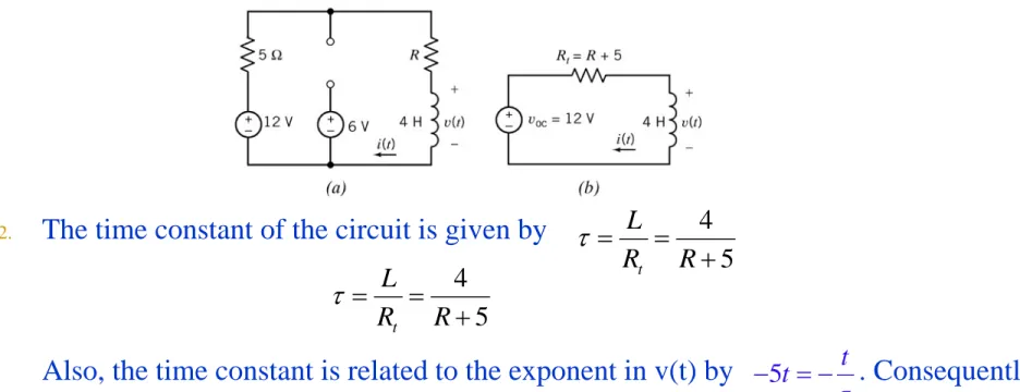
1. Figure 8.3-12a shows the circuit immediately after the switch opens.in Figure 8.3- 12b, the part of the circuit connected to the inductor has been replaced by its

Thévenin equivalent circuit.

2. The time constant of the circuit is given by

Also, the time constant is related to the exponent in v(t) by . Consequently

Solution(b)

4

t 5 L

R R

τ = = +

5 t

t τ

− = −

1 5

5 15Ω

4

R R

τ

= = + => =

4

t 5 L

R R

τ = = +

(40)

1. The inductor current is related to the inductor voltage by

2. Figure 8.3-13 show the circuit before the switch opens.

The inductor current is given by

In particular, i(0-)=0.4A. The current in an inductor is continuous, so i(0+)=i(0-).

Consequently,

3. Returning to the equation for the inductor current, after the switch opens we have

4. In summary,

Solution(c)

( ) 6 0.4A i t =15 =

5 5 5

0

1 1

( ) 4 0.4 ( 1) 0.4 0.6 0.2

4 5

t t t

i t = e⁻ ^τdτ + = e⁻ − + = − e⁻

∫

−

0

( ) 1 ^t ( ) (0)

i t v d i

L τ τ

=

∫

+

FIGURE 8.3-13

(0) 0.4A

i =

5

0.4 0

( ) 0.6 0.2 ^t 0

for t

i t e⁻ for t

 <

=  − ≥

(41)

Sequential Switching



Sequential switching occurs when a circuit contains two or more switches that change state at different instants.



Figure 8.4-1a is an example of sequential switching.

FIGURE 8.4-1

(42)

Sequential Switching (cont’d)

FIGURE 8.4-1

( ) 10 0

i t = A t <



Figure 8.4-1b shows the equivalent circuit that is appropriate for t<0.

(0 ) 10 i

⁻

= A

Before the switch changes state at time t=0.

(0 ) 10 i

⁺

= A

After the switch changes state at time t=0.

This is the initial condition at t=0.

[ ]

(43)

Sequential Switching (cont’d)

FIGURE 8.4-1

0 2

sc t

I = A and R = Ω



Figure 8.4-1c shows the equivalent circuit at 0< t <1 ms

3

2 10

3

1 10 1

t

2

L ms

τ = R = ×

⁻

= ×

⁻

= Time constant

( ) (0)

^t/

10

^t

0 1

i t = i e

⁻ ^τ

= e A

⁻

for < < t ms Inductor current

Immediately before t=1ms (1 ) 10

1

3.68 i

⁻

= e

⁻

= A Immediately after t=1ms

(1 ) 3.68 i

⁺

= A

[ ] [ ]

[ ]

[ ] [ ]

(44)

FIGURE 8.4-1

0 1

sc t

I = A and R = Ω



Figure 8.4-1d shows the

appropriate equivalent circuit.

3

2 10

3

2 10 2

t

1

L ms

τ = R = ×

⁻

= ×

⁻

= Time constant

( 0) / ( 1) / 2

( ) ( )

0 ^{t t}

3.68

^t

1

i t = i t e

^{− −} ^τ

= e

^{− −}

A for t > ms Inductor current

t

₀

denotes the time when the switch

changes state – 1ms in this example.



Figure 8.4-2 shows a plot of the inductor current.

FIGURE 8.4-2

[ ] [ ] [ ]

(45)

Sequential Switching (cont’d)



In some applications, switching occurs at prescribed voltage values rather than at prescribed times. Figure 8.4-3 a device, called comparator, that can be used to accomplish this kind of switching.

FIGURE 8.4-3

( )

^H

o

L

V if v v v t V if v v

+ −

 >

=   <

(46)

Sequential Switching (cont’d)



In figure 8.4-4, a comparator is used to compare the capacitor voltage to a threshold voltage V

_T

, Suppose

The input voltages of the comparator are so the output voltage of the comparator is

FIGURE 8.4-4

A T c

(0)

V > V > v

c

( )

T

v

₊

= v t and v

₋

= v

( ) ( )

( )

H c T

o

L c T

V if v t v v t V if v t v

 >

=   <

(47)



We know that the capacitor voltage of this first-order circuit will be

Let t

₁

denote the time when the comparator output voltage switches from V

_L

to V

_H

. Then v

_c

(t

₁

)=V

_T

, so

Solving for t

₁

gives

/( )

( ) ( (0) )

^{t RC}

c A c A

v t = V + v − V e

⁻

1/( )

[ (0) ]

^t ^RC

T A c A

V = V + v − V e

⁻

1

ln(

^c

(0)

^A

)

T A

v V

t RC

V V

= −

−

(48)

 Consider the circuit shown in Figure 8.4-5. The initial value of the capacitor voltage is v_c (0)=1.667 volts. What value of resistance, R, is required if the comparator is to switch from V_L=0 to V_H=5 volts at time t₁=1 ms

Example) Comparator Circuit

FIGURE 8.4-5

(49)

Solution

 Figure 8.4-5 shows a specific example of the circuit in Figure 8.4-4.

1. We get

2. Then, solving for R:

3 6 6

5 5

1 10 (1 10 ) ln 3 (1 10 ) ln(2) 10 5

3

R R

− − −

 − 

 

× = ×   = ×

 − 

 

 

3 6

1 10 1.44 ln(2) 10

R = ×

⁻ ₋

= k Ω

×

(50)

 In Figure 8.4-6, a comparator is used to compare the resistor voltage, v_R (t), to a threshold voltage, V_T. Suppose

Determine the time t₁ when the comparator output voltage switches from V_L to V_H

Example) Comparator Circuit

A T L

(0)

V > V > Ri

FIGURE 8.4-6

(51)

1. The resistor current is equal to the inductor current, so

2. The comparator does not disturb the first-order circuit consisting of the voltage source, resistor, and inductor. The inductor current is

3. Next, t₁ is the time when Ri_L(t₁)=V_T, so

4. Solving for t₁ gives

Solution

( ) ( )

R L

v t = Ri t

( / ) /

( ) ^A ( (0) ^A ) ^{R L} ^t

L L

V V

i t i e

R R

= + − −

1

ln( ^L(0) ^A)

T A

L Ri V

t R V V

= −

−

( / ) /1

( (0) ) ^{R L} ^t

T A L A

V =V + Ri −V e⁻

(52)

Stability of First-Order Circuits



Complete response



The circuit is stable

 When τ>0 , the natural response vanishes as t->0.



The circuit is unstable

 When τ<0, the natural response grows without bound as t->0.

 In most applications, the behavior of unstable circuits is undesirable and is to be avoided.



How can we design first-order circuits to be stable?

 R_t>0 is required to make a first-order circuit be stable.

( )

_n

( )

_f

( ) x t = x t + x t

( )

( ) / natural response ( ) (forced response)

t n

f

x t Ke x t

τ

= −

(τ = R C or_t τ = L R/ _t)

(53)

Example 8.5-1 Response of an Unstable First- Order Circuit



The First-order circuit shown in Figure 8.5-1a is at steady state before the switch closes at t=0. This circuit contains a dependent source and so may be unstable. Find the capacitor voltage, v(t), for t>0.

FIGURE 8.5-1

(54)

1. We calculate the initial condition from the circuit in Figure 8.5-2b.

1. Apply KCL to the top node of the dependent current source

2. Consequently, There is no voltage drop across the resistor and

2. Calculate the open-circuit voltage using the circuit in Figure 8.5-1c.

1. Writing a KVL equation, we get 2. We find

3. Applying Ohm’s law to the 10-kΩ resistor, we get

Solution

2 0

0 i i

i

− + =

= (0) 12V

v =

3 3

12 = ×(5 10 )× +i (10 10 ) (× × −i 2 )i 2.4mA

i = −

(10 10 ) (3 2 ) 24V VOC = × × −i i =

(55)

3. Calculate the Thévenin resistance using the circuit shown in Figure 8.5-1d.

1. Apply KVL to the loop consisting of the two resistors to get

2. Solving for the current,

3. Applying Ohm’s law to the 10-kΩ resistor, we get

4. The Thévenin resistance is given by

4. The complete response is

Solution

( ) ( )

3 3

0 = ×(5 10 )× +i 10 10× × I_T + −i 2i 2 _T

i = I

( )

3 3

10 10 2 10 10

T T T

V = × × I + −i i = − × ×I 10kΩ

T t

T

R V

= I = −

t 20ms

τ

= R C = −

( ) 24 12 ^t/ 20

v t = − e

(56)

Example 8.5-2 Designing First-Order Circuits to Be Stable



The circuit considered in Example 8.5-1 has been redrawn in Figure 8.5-2a, with the gain of the dependent source represented by the variable B. What restrictions must be placed on the gain of the dependent source to ensure that it is stable? Design this circuit to have a time constant of +20ms.

FIGURE 8.5-2

(57)

Solution

 Figure 8.5-2b the circuit used to calculate R_t 1. Applying KVL to the loop consisting of the two

resistors.

2. Solving for the current gives

3. Applying KCL to the top node of the dependent source, we get

4. Combining these equations, we get 5 10× 3× +i V_T = 0

3 0

10 10

T

i Bi V I

− + + − =

× 5 103

VT

i =

×

3 3

1 1

5 10 10 10 ^T ^T 0

B V I

 − +  − =

 × × 

 

(58)

Solution

5. The Thevenin resistance is given by

6. To obtain a time constant of +20ms requires

7. which in turn requires

10 103

2 3

T t

T

R V

I B

= = − ×

−

 B<3/2 is required to ensure that R_t is positive and the circuit is stable.

 Therefore B=1. This suggests that we can fix the unstable circuit by decreasing the gain of the dependent source from 2A/A to 1 A/A

3

3 10 10

10 10

2B 3

× = − ×

−

(59)

The Unit Step Source

 The Unit step forcing function as a function of time that is zero for t<t₀, and unity for t>t₀.

 Application of a constant-voltage source at t=t₀ using two switches both acting at t=t₀.

 Single-switch equivalent circuit for the step voltage source

 Symbol for the step voltage source

0 0

0

( ) 0 1

t t u t t

t t

 <

− =  >

0 0

( ) ( )

v t =V u t −t

(60)

The Unit Step Source

 A pulse signal has a constant nonzero value for a time duration of Δt=t₁-t₀

 Pulse source

 Two-step voltage sources

0 0 0 1

0

0 0 1

1

( ) ( ) ( )

0 0

v t V u t t V u t t t t

V t t t

t t

= − − −

 <

=  < <

 <



(61)

The Unit Step Source

 Let us consider the application of a pulse to an RL circuit as shown in Figure 8.6- 7. Here we let t₀=0. The pulse is applied to the RL circuit when i(0)=0.

 Since the circuit is linear, we may use the principle of superposition, so that where i₁ is the response to V₀u(t) and i₂ is the response to V₀u(t-t₁)

 The response of an RL circuit to a constant forcing function applied at t=t_n is

where τ=L/R.

FIGURE 8.6-7

1 2

i = + i i

( ) /

0 (1 ^{t t}ⁿ ) when _n

i V e t t

R

τ

= − − − >

(62)

The Unit Step Source

 The two solutions to the two-step sources are

 Adding the responses, we have

 The response at t=t1 is

 If t₁ is greater than τ, the response will approach V₀/R before starting its decline, as shown in Figure 8.6-8. The response at t=2t₁ is

1

0 / 1

( ) / 0

2 1

(1 ) 0

(1 )

t

t t

i V e when t

R

i V e when t t

R

τ

−

− −

= − ≥

= − − >

0 /

1

/ /

0

1

(1 ) 0

( 1)

t

t t

V e t t

i R

V e e t t

R

τ

τ τ

−

 − < ≤

= − − >



1/ 0

( )1 V (1 ^t )

i t e

R

τ

= − −

1 1 1 1

2( / ) / / 2( / )

0 0

(2 )1 V ^t ( ^t 1) V ( ^t ^t )

i t e e e e

R R

τ τ τ τ

− − − −

= − = − FIGURE 8.6-8

(63)

Example 8.6-1 First-Order Circuit



Figure 8.6-9 shows a first-order circuit. The input to the circuit is the voltage of the voltage source, v

_s

(t). The output is the current of the inductor, i

₀

(t). Determine the output of this circuit when the input is v

_s

(t)=4-8u(t) [V].

FIGURE 8.6-8

(64)

Solution

1. The response of the first-order circuit will be

2. Circuits used to calculate the steady-state reponse

(a)before t=0 (b) after t=0

3. The value of the constant a is determined from the time constant τ.

(0) 0(0)

0.2

i A Be a A B

A B A

= + − = +

+ =

( ) 0( )

= 0.2A

i A Be a A

A

∞ = + − ∞ =

−

0.4A B =

1

t

L a = =τ R

( ) ^at 0

i to = +A Be⁻ for t >

(65)

Solution

4. Figure 8.6-11 shows the circuit used to calculate R_t.

Therefore,

5. Substituting the values of A, B and a gives

t 20

R = Ω

20 1

10 2

a = = s

0 2

0.2 0

( ) 0.2 0.4 ^t 0

A for t

i t e⁻ A for t

 ≤

= − + ≥

FIGURE 8.6-11 [ ]

[ ]

(66)

Example 8.6-2 First-Order Circuit



Figure 8.6-12 shows a first-order circuit. The input to the circuit is the voltage of the voltage source, v

_s

(t). The output is the voltage across the capacitor, v

_o

(t). Determine the output of this circuit when the input is v

_s

(t)=7-14u(t)V.

FIGURE 8.6-12

(67)

Solution

1. The response of the first-order circuit will be

2. Circuits used to calculate the steady-state reponse

(a)before t=0 (b) after t=0

3. The value of the constant a is determined from the time constant τ.

(0) 0(0)

5 7 4.38V 3 5

v A Be a A B

A B

= + − = +

+ = × = +

( ) 0( )

= 5 ( 7) 4.38V 3+5

v A Be a A

A

∞ = + − ∞ =

× − = −

8.76V B =

1

R Ct

τ

= =

( ) ^at 0

v to = +A Be⁻ for t >

(68)

Solution

4. Figure 8.6-14 shows the circuit used to calculate R_t.

Therefore,

5. Substituting the values of A, B and a gives (5)(3)

1.875

t 5 3

R = = Ω

+

3

1 1

(1.875)(460 10 ) 1.16

a = ⁻ = s

×

0 1.16

4.38V 0

( ) 4.38 8.76 ^tV 0

for t

v t e⁻ for t

− ≤

= 

− + ≥



FIGURE 8.6-14

(69)

The Response of a First-Order Circuit to a Nonconstant Source

 The differential equation an RL or RC circuit is represented by the general form

 Consider the derivative of a product of two terms such that

 The term within the parentheses on the right-hand side of Eq.8.7-2 is exactly the form on the left-hand side of Eq.8.7-1.

Therefore,

 Integrating both sides of the second equation, we have ( ) ( ) ( )

dx t ax t y t

dt + =

(dx ) ât ât d ( ât) ât

ax e ye or xe ye

dt + = dt =

( ât) ât ât ( ) ât

d dx dx

xe e axe ax e

dt = dt + = dt + (8.7-2)

(8.7-1)

at at

xe =

∫

ye dt +K

(70)

The Response of a First-Order Circuit to a Nonconstant Source

 Therefore,

 For the case where the source is a constant so that y(t)=M, we have

 Consider the case where y(t), the forcing function, is not a constant.

(8.7-2) (8.7-1)

at at at

x =e⁻

∫

ye dt +Ke⁻

natural response :

forced response : /

at at at at

f n

at n

f

x e M e dt Ke M Ke x x

a x ke

x M a

− − −

−

= + = + = +

=

∫

( ) ( )

natural response : forced response : 1

at n

bt

at bt at at a b t at a b

f

x ke

x e e e dt e e dt e e e

a b a b

−

− − + − +

=

= = = =

+ +

∫ ∫

(71)

Example 8.7-1 First-Order Circuit with Nonconstant Source



Find the current i for the circuit of Figure 8.7-1a for t>0 when

Assume the circuit is in steady state at t=0

^-

FIGURE 8.7-1 10 2^t ( )V vs = e u t⁻

(72)

Solution

1. We expect i_f to be

2. Writing KVL arround the right-hand mesh, we have

3. Substituting , we have

Hence, B=5 and

4. The natural response can be obtained by considering the circuit shown in Figure 8.7-1b. This is the equivalent circuit after the switch opens. The natural response is

4 10 2^t s

di di

L Ri v or i e

dt dt

+ = + = −

2t

if = Be⁻

2 2 2 2 2

2Be⁻ ^t 4Be⁻ ^t 10e⁻ ^t or ( 2B 4 )B e⁻ ^t 10e⁻ ^t

− + = − + =

2t

if = Be⁻

5 2^t

if = e⁻

(R L t_t/ ) 4t

in = Ae⁻ = Ae⁻

(73)

Solution

5. The complete response is

6. The constant A can be determined from the value of the inductor current at time t=0. The initial inductor current, i(0), can be obtained by considering the circuit shown in Figure 8.7-1c. This is the equivalent circuit that is appropriate before the switch opens.

7. From Figure 8.7-1c 8. Therefore, at t=0

9. Therefore,

(0) 10 2 i = 5 = A

4 2

t 5 t

n f

i = + =i i Ae⁻ + e⁻

4 0 2 0

(0) 5 | 5

2 5

3

i Ae e A