Vol. 70, No. 8, August 2020, pp. 667∼674 http://dx.doi.org/10.3938/NPSM.70.667
Calculation of the off-axes Magnetic Field for Finite-length Solenoids
Taehun Jang
Department of Physics, Kyungpook National University, Daegu 41566, Korea
Yun Kyung Seo · Sang Ho Sohn
∗Department of Science Education, Graduate School, Kyungpook National University, Daegu 41566, Korea
JoongWoo Jung
Haknam High School, Daegu 41420, Korea (Received 12 June 2020 : accepted 29 June 2020)
In this study, we derived an approximate analytic function for the off-axis magnetic field of a finite-length solenoid by using the magnetic vector potential of a circular current loop. We verified that the derived analytic function reduced to a well-known magnetic field formula on the vertical axis of the solenoid and also inferred the magnetic field on the horizontal axis of the solenoid.
Furthermore, we investigated the magnetic field at arbitrary points satisfying the approximate conditions through a simulation performed using Wolfram Mathematica.
Keywords: Magnetic field, Off-axes solenoid, Analytic function, Mathematical simulation
I. Introduction
A solenoid is a coil that is wound many times along an axis, and a magnetic field is generated around the solenoid when a current flows through it. When a large current flows through a solenoid, a strong magnetic field is generated inside it. Therefore, solenoids are used as strong magnets. Furthermore, because of magnetic forces acting on the ends of a solenoid, it is also used as an electrically controlled valve. Although solenoid is employed in commonly used devices such as micro- phones, speakers, transformers, and metal detectors, stu- dents learn about solenoids in high school. In high school curriculums, an exploration activity involving the obser- vation of how a compass needle changes direction around a solenoid as the current flowing through the solenoid changes is introduced, and an experiment in which the magnetic field of a solenoid is measured as a function of currents is included [1]. In university textbooks, a re- fined formula for the magnetic field on the central axis
∗E-mail: [email protected]
of a finite-length solenoid is derived. In particular, the magnetic field on the central axis is uniform when the solenoid is infinitely long [2].
A recent study considered a magnet to be a solenoid and theoretically calculated the magnetic force between the magnet and a solenoid on the basis of the mutual inductance effect [3]. While magnetic fields produced by solenoids have been studied in previous works [4–6], most of the studies investigated magnetic fields on the vertical central axis, namely z-axis of the cylindrical co- ordinate. Knowledge of the magnetic field at a point away from a solenoid axis is useful for determining the electromotive force induced on the solenoid by a magnet moving around the solenoid as well as the magnetic force between the magnet and the solenoid. Accordingly, the- oretical formulas for magnetic fields on the off-axis of a solenoid are required and several previous studies have used the Biot-Savart law [7], magnetic scalar potential [8], or magnetic vector potential [9] to determine the off-axis magnetic field. However, because the formulas
This is an Open Access article distributed under the terms of the Creative Commons Attribution Non-Commercial License (http://creativecommons.org/licenses/by-nc/3.0) which permits unrestricted non-commercial use, distribution, and reproduction in any medium, provided the original work is properly cited.
obtained by these studies contain elliptic integrals, the analytic function is not available.
In this study, an approximate analytic function was derived for the magnetic field at arbitrary points of an off-axis of solenoid. In addition, the magnetic fields at points within an approximate limit around a solenoid were obtained via a simulation using Wolfram Mathe- matica, and they are discussed here. The analytic func- tions derived in the present study for off-axis magnetic fields for a solenoid can be useful to determine the mag- netic field near the central axis of electromagnets and far the surface of permanent magnets, which are considered as solenoids, as well as the magnetic force on a magnet moving outside a solenoid.
II. Theoretical calculations
In this study, the following theoretical approach was used for calculating the magnetic field at an arbitrary point of off-axis of solenoid. First, we considered the solenoid as a collection of circular current loops and cal- culated the vector potentials Aφ(r, θ) and Aφ(ρ, z) at arbitrary positions (r, θ) and (ρ, z) for a single circu- lar current loop. The elliptic integrals appearing in the equations were represented as power series by considering appropriate approximations to obtain the analytic func- tion for Aφ. Second, we obtained the magnetic field of the solenoid by first determining the magnetic field of a single circular current loop from the relation B =∇ × A and then integrating it along the z-axis.
The magnetic field formula derived was validated by comparing the magnetic fields on the central z-axis ob- tained from the formula with those obtained for the z- axis from a well-known magnetic field formula. Magnetic fields at points on the horizontal axis at z = 0 were also determined from the derived formula. Finally, a sim- ulation was performed using Wolfram Mathematica to calculate magnetic fields at arbitrary points around the solenoid.
1. Magnetic fields B(r, θ) and B(ρ, z) at arbitrary points (r, θ) and (ρ, z) around a circular current loop
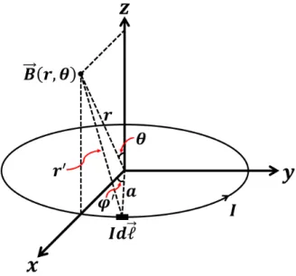
Fig. 1. (Color online) Magnetic field B(r, θ) at arbitrary points (r, θ) on a circular current loop
Figure 1 shows the magnetic field B(r, θ) at arbitrary point (r, θ) on a circular current loop.
In the Fig. 1, the vector potential A can be defined as
A = µ0I 4π
∫ d⃗l
r′ (1)
Furthermore, r′ and d⃗l are given by
r′= (r2+ a2− 2ar sin θ cos φ′)1/2
d⃗l = a(− sin φ′x + cos φˆ ′y)dφˆ (2) and the vector potential A can be expressed as
A = µ0Ia 4π
∫ 2π 0
(− sin φ′x + cos φˆ ′y)dφˆ ′
(a2+ r2− 2ar sin θ cos φ′)1/2 (3) The azimuthal integration path of the magnetic field at the periphery of the circular current loop is symmetric about φ′ = 0. Therefore, the x-component disappears and only the y-component of Aφ remain [10].
Aφ(r, θ) =µ0I a 4π
∫ 2π 0
cos φ′
(a2+ r2− 2ar sin θ cos φ′)1/2dφ′ (4) Substituting φ′ = 2φ + π in this equation gives dφ′ = 2dφ and φ = −π2 ∼ +π2, and the use of the relation k2= a2+r4ar sin θ2+2ar sin θ yields
(a2+ r2− 2ar sin θ cos φ′)1/2
=(
a2+ r2+ 2ar sin θ)1/2
(1− k2sin2φ)1/2
and
cos φ′ = cos(2·φ′
2 ) = 1− 2 sin2φ′
2 = 1− 2 sin2(φ +π 2)
= 1− 2 cos2φ = 1− 2(1 − sin2φ) = 2sin2φ− 1 (5) Therefore, equation (4) can be expressed as
Aφ(r, θ) =µ0I a 4π
4
(a2+ r2+ 2ar sin θ)1/2
×
∫ π/2 0
2sin2φ− 1 (1− k2sin2φ)1/2dφ
(6)
Furthermore, we can use the mathematical relation sin2φ =1−(1−kk22sin2φ) to modify equation (6) as
∫ π2
0
2sin2φ− 1
(1− k2sin2φ)12 dφ =
∫ π/2 0
2
{1−(1−k2sin2φ) k2
}− 1
(1− k2sin2φ)1/2 dφ
=
∫ π/2 0
(k22 − 1)
(1− k2sin2φ)1/2dφ−
∫ π/2 0
2
k2(1− k2sin2φ) (1− k2sin2φ)1/2dφ
= (2
k2 − 1)K(k2)− 2 k2E(k2)
(7) where
K(k2) =
∫ π2
0
dφ
(1− k2sin2φ)1/2 (8)
E(k2) =
∫ π2
0
(1− k2sin2φ)1/2dφ (9) Equations (8) and (9) are the complete elliptic integrals of the first and second kind, respectively. Vector poten- tial Aφ(r, θ) can be expressed as
Aφ(r, θ) =µ0I a 4π
4
(a2+ r2+ 2ar sin θ)1/2
×
[(2− k2)K(k2)− 2E(k2) k2
] (10)
Equation (10) is a formula for calculating the magnetic field at arbitrary point (r, θ) of a circular current loop, but it is difficult to use because the elliptic integral is not in a closed form (i.e., it is not in the form of an analytic function). Moreover, in the case of solenoids, we must integrate equation (10) in the z-axis direction, in which case even the elliptic integration of the third kind should be considered [9].
In this study, the aim was to obtain the magnetic field at arbitrary points around a solenoid. In general, the
magnetic field inside an infinitely long solenoid is al- most similar to that on the central axis, and it is known to be very weak near the outside of the solenoid [11].
For a finite-length solenoid, it is possible to expand the elliptic integrals in equation (10) under the conditions r≫ a, a ≫ r, or sin θ ≈ 0 as [12]
K(k2) = 1 + k2 4 +9k4
64 +· · · (11) and
E(k2) = 1−k2 4 −3k4
64 +· · · (12) When only the term k2 considered, the value of the ex- pression in the square brackets of Equation (10) is k2/16.
Therefore, the vector potential can be expressed as Aφ(r, θ) = µ0I
4
a2r sin θ
(a2+ r2+ 2ar sin θ)3/2 (13) In cylindrical coordinates, equation (13) can be trans- formed as
Aφ(ρ, z) = µ0I 4
a2ρ
(ρ2+ z2+ a2+ 2aρ)3/2 (14) From the relation B =∇×A, the magnetic field compo- nents Br, Bθ, and Bφof the magnetic field B in spherical coordinates can be expressed as
Br= 1 r sin θ
∂
∂θ(sin θAφ(r, θ))
= µ0I a2sin θ 4
(2r2+ 2a2+ ar sin θ) (a2+ r2+ 2ar sin θ)5/2
(15)
Bθ=−1 r
∂
∂r(rAφ(r, θ))
= µ0I a2sin θ 4
(r2− 2a2− ar sin θ) (a2+ r2+ 2ar sin θ)5/2
(16)
Bφ= 0 (17)
In cylindrical coordinate, the magnetic field components can be expressed as
Bρ=−∂Aφ(ρ, z)
∂z = 3µ0I a2ρz
4(ρ2+ z2+ a2+ 2aρ)5/2 (18)
Bz =1 ρ
∂
∂ρ(ρAφ(ρ, z))
=µ0I a2 4
2(ρ2+ z2+ a2+ 2aρ)− 3ρ(ρ + a) (ρ2+ z2+ a2+ 2aρ)5/2
(19)
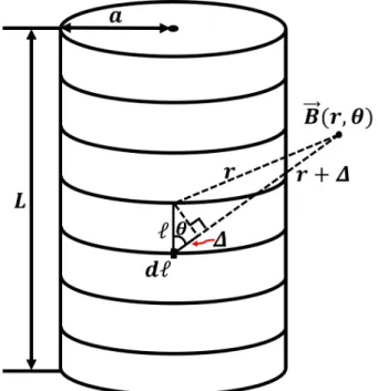
Fig. 2. (Color online) Magnetic field B(r, θ) at arbitrary points (r, θ) around a solenoid with N turns
If the solenoid is considered as a combination of circular current loops, B(r, θ) and B(ρ, z) can be derived from the relation B =∇ × A after integrating equations (13) and (14) along the z-axis. However, because integrating equations (15), (16), (18), and (19) along the z-axis is more convenient for the calculation of magnetic field, we adopted this approach in this study.
2. Magnetic fields B(r, θ) and B(ρ, z) at arbitrary points (r, θ) and (ρ, z) around a solenoid
Figure 2 shows the magnetic field B(r, θ) at arbitrary point (r, θ) around a solenoid with N turns. l denotes the distance from the center of the solenoid to the field source. Also we define the vertical axis as z-axis of a cylindrical coordinate while the horizontal axis as ρ-axis.
Substituting r + ∆ = r + l cos θ and NLIdl(= nIdl) equations (15) and (16) gives
dBr=µ0nIa2cos θ 4
× [2(r + l cos θ)2+ a(r + l cos θ) sin θ + 2a2] [(r + l cos θ)2+ 2a(r + l cos θ) sin θ + a2]5/2dl
(20)
dBθ=µ0nIa2sin θ 4
× [(r + l cos θ)2− a(r + l cos θ) sin θ − 2a2] [(r + l cos θ)2+ 2a(r + l cos θ) sin θ + a2]5/2dl
(21) By replacing r + l cos θ ≡ t and integrating equations (20) and (21) from−L/2 to L/2, we can derive
Br(r, θ) =µ0nI a2
4 [P + Q + R] (22)
where
P = 2p3
3(2pa sin θ + a2)(p2+ 2pa sin θ + a2)3/2
− 2q3
3(2qa sin θ + a2)(q2+ 2qa sin θ + a2)3/2 (23)
Q = a sin θ
3(q2+ 2qa sin θ + a2)3/2− a sin θ
3(p2+ 2pa sin θ + a2)3/2 (24)
R = 2pa2(2p2+ 6pa sin θ + 3a2) 3(2pa sin θ + a2)2(p2+ 2pa sin θ + a2)3/2
− 2qa2(2q2+ 6qa sin θ + 3a2) 3(2qa sin θ + a2)2(q2+ 2qa sin θ + a2)3/2
(25)
Here, p and q are given by r + L2cos θ and r−L2 cos θ, respectively.
For the vertical central axis (r = z, θ = 0) of the solenoid, equation (22) reduces to
Br(r, θ)⇒
Bz(z, 0) = µ0nIa2
4 [(P )r=z,θ=0+ (Q)r=z,θ=0+ (R)r=z,θ=0]
= µ0nI 2
[
z +L2
((z +L2)2+ a2)1/2− z−L2 ((z−L2)2+ a2)1/2
]
(26) which is a well-known formula for the magnetic field on the vertical central axis [11].
On the horizontal central axis (r = ρ, θ = π/2), equa- tion (22) becomes
Bρ(ρ,π
2) = 0 (27)
since the term (P )r=ρ,θ=π/2 + (Q)r=ρ,θ=π/2 + (R)r=ρ,θ=π/2 becomes zero.
Thus, on the horizontal central axis, the magnetic field has only the vertical components since only Bz values exist.
Similarly, equation (21) can be integrated using the integral table to obtain
Bθ(r, θ) = µ0nIa2tan θ 4
[P
2 − Q − R ]
(28) On the vertical central axis (r = z, θ = 0), equation (28) becomes 0 because tan θ = 0
Bθ(r = z, θ = 0) = 0 (29) and on the horizontal central axis (r = ρ, θ = π/2), equation (28) becomes
Bθ(r = ρ, θ = π/2) = µ0Ina2tan(π/2)
4 [0− 0 − 0] (30) Equation (30) is an indeterminate form of ∞ × 0. so we substituted the limita-
tion from lim
θ→π/2tan θ[
P (θ)
2 − Q(θ) − R(θ)] to lim
θ→π/2
[P (θ)2 −Q(θ)−R(θ)]
cot θ to differentiate the equation by applying l’Hôpital’s rule, thereby obtaining
Bθ(r = ρ, θ = π/2)
=µ0nI
4 [ −3ρ4
(ρ2+ a2)5/2 + 5ρ2
(ρ2+ a2)3/2− 2
(ρ2+ a2)1/2]L (31) which is a function of ρ.
Using equations (22) and (28), we can obtain the mag- netic field B(r, θ)
B(r, θ) = Br(r, θ)ˆr + Bθ(r, θ)ˆθ (32) Thus, we can obtain the magnetic field of a solenoid at arbitrary point (r, θ). Equation (32) can be used to find the electromagnetic force acting on a magnet traversing a solenoid.
Meanwhile, to determine the B (ρ, z) for a solenoid, we can write equation (18) as
dBρ= 3µ0nIa2ρ(z− z′)
4[ρ2+ (z− z′)2+ a2+ 2aρ]5/2dz′ (33) and integrate equation (33) after substituting a2+ 2aρ = c2
Bρ(ρ, z) = 3µ0nI a2ρ 4
∫ L2
−L2
z− z′
ρ2+ (z− z′)2+ c2dz′
=µ0nI a2ρ 4
[ 1
(s2+ ρ2+ c2)3/2− 1
(t′2+ ρ2+ c2)3/2 ]
(34)
where s = z−L2 and t′ = z +L2. Because z is zero on the horizontal central axis, in equation (34), Bρ = 0 (i.e., only Bz exists). From equation (19), we have
dBz= µ0nIa2 4
2[ρ2+ (z− z′)2+ c2]− 3ρ(ρ + a) [ρ2+ (z− z′)2+ c2]5/2 dz′
(35) This equation can be integrated using the integral table to obtain
Bz(ρ, z) =µ0nI a2 4
∫ L
2
−L2
2[ρ2+ (z− z′)2 + c2]− 3ρ(ρ + a) [ρ2+ (z− z′)2+ c2]5/2 dz′
=µ0nI a2 4
[−2c2s3+ (ρ4− a4+ ρ2a2+ ρ3a + 3ρa3)s (ρ2+ c2)2(s2+ ρ2+ c2)3/2
− −2c2t′3+ (ρ4− a4+ ρ2a2+ ρ3a + 3ρa3)t′ (ρ2+ c2)2(t′2+ ρ2+ c2)3/2
]
(36) For the vertical central axis (ρ = 0), we can derive from equation (36) as
Bz(ρ = 0, z)
= µ0nI 2
[ t′
(t′2+ a2)1/2 − s (s2+ a2)1/2
]
= µ0nI 2
[ (z + L2)
((z +L2)2+ a2)1/2− (z−L2) ((z−L2)2+ a2)1/2
]
(37) which is a well-known expression for the magnetic field on the vertical central axis of a solenoid [11].
Finally, we can obtain B(ρ, z) from equations (34) and (36):
B(ρ, z) = Bρ(ρ, z) ˆρ + Bz(ρ, z)ˆz (38) Using this equation, we can determine the magnetic field at arbitrary point (ρ, z). Equation (38) can also be used to obtain the electromagnetic force acting on a small magnet moving on the vertical central axis of a solenoid.
As shown in equations (22), (28), (34), and (36), all com- ponents of magnetic fields of a finite solenoid depend on n, a, and L. This dependence has been also reported in the earlier numerical studies [8,9].
III. Results and discussion
While equations (22) and (28) are useful for determin- ing the magnetic field at arbitrary point (r, θ), the equa- tions in cylindrical coordinates are more helpful since
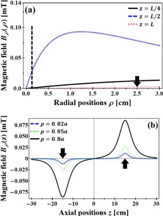
Fig. 3. (Color online) Estimation of Bz(ρ, z) and Bρ(ρ, z) along the horizontal and vertical axes of a solenoid.
a solenoid has a cylindrical shape. Therefore, in this study, we used equations (34) and (36) for the estimation of the magnetic field around a solenoid. We performed a simulation using Wolfram Mathematica to determine the magnetic field on the horizontal and vertical axes of a solenoid, as shown in Fig. 3. The radius, length, number of turns, and applied current for the solenoid were a = 2.5 cm, L = 30 cm, N = 600, and I = 1 A, respectively.
Figure 4 (a) shows Bρ(ρ) at the positions z = L/4, L/2, and L. Clearly, Bρ(ρ, z) becomes zero on the vertical central axes (ρ = 0). Bρ(ρ) shows rela- tively large values at the edge (z = L/2) of the solenoid and is very weak inside (z = L/4). But, the data for z = L/4, L/2 cannot represent exact magnetic fields Bρ(ρ) because it was not obtained within the approx- imate limit r ≫ a, a ≫ r, or sin θ ≈ 0 (left side of the black dotted vertical line in Fig. 4(a)). In the circular coils and solenoids, Bρ(ρ) is expected to have a peak- like maximum of the magnetic field at the coil position (noted by an arrow in Fig. 4 (a) but Bρ(ρ) is almost zero within the approximate limit. Figure 4 (b) shows Bρ(z) at the positions ρ = a/50 (= 0.02a) , a/20(= 0.05a), and 4a/5(= 0.8a).Bρ(z) at the positions ρ = a/50 and a/20 shows the peak-like narrow distributions at the edge po- sitions (noted by two arrows in Fig. 4 (b) while it shows
Fig. 4. (Color online) (a) Bρ(ρ, z) at the positions z = L/4, L/2 and L, (b) Bρ(z) at the positions ρ = a/50, a/20 and 4a/5.
the broad ones at the position ρ = 4a/5. These nar- row field distributions at the edges have been reported in the earlier study [8] and represent the relatively exact fields whereas the broad ones cannot tell reliable mag- netic values because the positions ρ = 4a/5 is not within the approximate limit, r≫ a, a ≫ r, or sin θ ≈ 0. Thus, equation (34) holds good for the regions near the z axis or far away from a solenoid.
Figure 5 shows Bz(z) at the positions ρ = 0, a/50, a/20, and 2a. Evidently, on the vertical central axis, Bz(ρ = 0, z) coincides with the known magnetic field distribution. For small ρ-values, Bz(z) tends to very slightly decrease, compared to Bz(ρ = 0, z). In Fig.
5, Bz(z) inside the solenoid decreases by about 0.07 mT in each of three cases. It is noted that Bz(ρ = a/50, z) approaches to Bz(ρ = 0, z) on the vertical central axis at an error 4% and Bz(ρ = a/20, z) is about 90% of Bz(ρ = 0, z). In addition, as is well known, the magnetic fields at the edge (noted by an arrow in Fig. 5) of the solenoid become halves of those in the center in all cases.
Fig. 5. (Color online) Bz(z) at the positions ρ = 0, a/50, a/20 and 2a.
Fig. 6. (Color online) Bz(ρ) at the positions z = 0, L/4, L/2 and L.
This means that the derived formula equation (36) is a useful approximation for calculating near-axis magnetic fields of a finite solenoid even if they are not absolutely exact. Outside the solenoid, Bz(z) is very small but not zero.
Figure 6 shows Bz(ρ) at the positions z = 0, L/4, L/2, and L. ρ values are selected within the approximate limit, r ≫ a, a ≫ r, or sin θ ≈ 0, namely ρ < a/20.
The slight variations of Bz(ρ) according to ρ proba- bly originate from the approximate error or the natu- ral properties of the finite solenoid as argued in pre- vious articles [8,9]. It is noted that as is well known, Bz(ρ, z = L/2)/Bz(ρ, z = 0) is 1/2 in Fig. 6.
Thus, we present useful analytic functions that can be used for determining the magnetic field at arbitrary points around a solenoid under the approximate condi- tions r≫ a, a ≫ r, or sin θ ≈ 0.
The magnetic fields should be measured for the con- ditions (r≫ a, a ≫ r, or sin θ ≈ 0) used for deriving the
analytic function in this study to compare with the val- ues obtained from the formula. Such measurements can be obtained by using a magnetic field sensor, which can be moved in the ρ- and z-direction. In the near future, we plan to conduct a study for experimentally measur- ing the magnetic field of a solenoid with an appropriate device.
IV. Conclusion
Using the magnetic field vector potential of a circu- lar current loop and integrating it along the azimuthal direction, we derived approximate analytic functions for obtaining the magnetic field of a solenoid at an arbi- trary off-axis points under the approximate conditions r ≫ a, a ≫ r, or sin θ ≈ 0 of a finite solenoid. The derived analytic function of magnetic field reduces to a well-known magnetic field formula on the z-axis, showing the validity of the derived analytic function. All compo- nents of magnetic fields of a finite solenoid depend on n, a, and L.
The magnetic fields at arbitrary off-axis points within an approximate limit for a solenoid were estimated via simulations by using Wolfram Mathematica. A very weak and almost constant Bρ(ρ, z) was observed in the regions far away from the solenoid. Furthermore, Bz(ρ, z) is not constant inside the solenoid, but very slightly decreases with respect to ρ positions within the approximate limit and that the magnetic field is small but nonzero outside a finite-length solenoid. The reason for the small radical variation of Bz(ρ, z) is unclear if the approximate error or the natural properties of the finite solenoid and experimental studies are needed for it.
In conclusion, we present the limited but useful ana- lytic functions for determining the magnetic field at arbi- trary points near the z axis or far away from a solenoid.
The analytic functions for the magnetic field derived in this study are expected to be useful for determining the magnetic field near the central z-axis of electromagnets and far the surface of permanent magnets, which are con- sidered as solenoids, as well as the magnetic force acting on a magnet moving outside a solenoid.
REFERENCES
[1] Youngmin Kim et al., Physics Ⅱ (Kyohak Publica- tion, Seoul, 2015).
[2] David J. Griffiths, Introduction to Electrodynamics (Prentice Hall, New Jersey, 1999).
[3] J. W. Jung, Master thesis (Kyungpook National University, 2019.).
[4] N. Derby, S. Olbert, Am. J. Phys. 78, 229 (2010).
[5] V. Labinac, N. Erceg, and D. Kotnik-Karuza, Am.
J. Phys. 74, 621 (2006).
[6] J. M. Camacho, V. Sosa, Revista mexicana fisica E 59, 8 (2013).
[7] S. Basu, S. S. Pany, P. Bannerjee and S. Mitra, Journal of Electromagnetic Analysis and Applica- tions 5, 371 (2013).
[8] S. R. Muniz, V. S. Bagnato and M. Bhattacharya, Am. J. Phys. 83, 513 (2015).
[9] E. E. Callaghan, S. H. Maslen, NASA Technical note No. 19980227402 (1960).
[10] J. D. Jackson, Classical Electrodynamics 3rd ed.
(John Wiley & Sons, NewYork, 1998).
[11] P. Lorrain, D. Corson, Introduction to Electromag- netic fields and waves (W. H. Freeman and Com- pany, London, 1970).
[12] V. N. Belykh, J. Appl. Ind. Math. 6, 410 (2012).