Print ISSN: 2288-4637 / Online ISSN 2288-4645 doi:10.13106/jafeb.2020.vol7.no3.101
Overconfidence Bias, Comparative Evidences between Vietnam and Selected ASEAN Countries
Dzung Tran Trung PHAN*, Van Hoang Thu LE**, Thanh Thi Ha NGUYEN***
Received: January 01, 2020 Revised: February 01, 2020 Accepted: February 06, 2020.
Abstract
The study aims to investigate the existence of overconfidence bias in Vietnam, Thailand, and Singapore. This paper focuses on the Vietnam Stock Market and other two countries of ASEAN, namely Singapore and Thailand. Data was collected over the period from January 1, 2014 to December 31, 2018, daily returns for each of the securities. This paper uses the time series method, namely ADF test, Granger Causality and VAR approach to find evidences of the overconfidence effect in Vietnam in relation to some ASEAN markets. The results show similarities between the observed countries with slight variations, with focus on Vietnam market. In general concrete evidences of overconfidence were found in both Vietnamese and Singaporean markets, in which Singaporean investors show higher degree of overconfidence than Vietnamese investors.
Overconfidence is not as clear in Thai market, however a direct causal link from increased returns to increased investor confidence was found.
From the model deployed in the paper, there are reasons to conclude that Thai investors are under-confident. The findings of the study shed lights into the existence of overconfidence bias in Vietnam, Thailand, and Singapore on a comparative basis, provide more insights and implications for future research in this new and rising field of research.
Keywords: Behavioral Finance, Overconfidence, Vietnam, ASEAN JEL Classification Code: G10, G11, G41
1.Introduction 1718
The assumption that all investors are rational is the basis for the conventional asset pricing models. However, more and more empirical evidences suggest that those models cannot explain many stylized facts observed in the real securities market. It results in growing interest in finding reasons why conventional asset-pricing model does not hold at all time. One potential idea that has grown into a whole branch of study called Behavioural Finance is that investors are not rational when making financial decisions,
*First Author and Corresponding Author. Vice Dean, Faculty of Banking and Finance, Foreign Trade University, Vietnam [Postal Address: 91 Chua Lang Street, Dong Da District, Ha Noi, 100000, Vietnam] Tel.: (+84) 0904216521, Email: [email protected]
**Research Scholar, Foreign Trade University, Vietnam.
Email: [email protected]
***Lecturer, Faculty of Banking and Finance, Foreign Trade University, Vietnam. Email: [email protected]
© Copyright: The Author(s)
This is an Open Access article distributed under the terms of the Creative Commons Attribution Non- Commercial License (https://creativecommons.org/licenses/by-nc/4.0/) which permits unrestricted non- commercial use, distribution, and reproduction in any medium, provided the original work is properly cited.
which violates the most fundamental assumption of traditional finance theories. In this field of study, many cognitive as well as emotional biases affecting investors‟
way of thinking and feeling have been put forward as explanation for anomalies in individual investment decisions and the performance of financial markets.
Overconfidence is one of the main biases in Behavioural Finance.
Featuring the nature of an immature market where there are numerous individual investors and speculation frequently happens, Vietnam stock market is subject to behavioural factors, especially investors‟ overconfidence.
Therefore, the study of behavioural psychology proves to be necessary to the market and investors, particularly in the current period when Vietnam is now facing with various growth opportunities: The Comprehensive and Progressive Agreement for Trans-Pacific Partnership (CPTPP) entered into force, the Vietnam – EU Free Trade Agreement (EVFTA) has been finalized and will soon be signed, The US – China trade tension brings Vietnam advantages. These promising news can potentially trigger irrational beliefs of investors, drive investor sentiment and make them overconfident about the performance of Vietnam stock
market. By realizing the existence of this bias, investors may return to their rational behaviour, which helps prevent consequences on the market level such as abnormal market returns and volatility. This is also the concern of the regulatory authorities if they want to ensure that Vietnam stock market functions efficiently. This would be an important task for the country as Vietnam has set target that the stock market could be upgraded to secondary emerging status in March 2020 by FTSE Russell after the revised securities law is approved in the eighth session of the National Assembly's 14th legislature. There were discussions of the importance of economic integration to development (Bong & Premaratne, 2019; Hur & Park, 2012; Tai & Lee, 2009; Wong & Chan, 2003)
The research is put in perspective and comparative basis with two ASEAN stock markets, which are Singapore and Thailand market. All three countries share similar characteristics in terms of economic, political and social conditions but growth paces of their economies and securities markets are varying. It can provide with meaningful comparisons among these three ASEAN markets and some lessons for improving the efficiency of Vietnam stock market. It is found by various studies, that economic integration and similar economic condition could generate a cross-affect situation between countries (Lee &
Zhao, 2014), with the short run causality from Japan and Korea to Chinese stock price, while Valadkhani and Chancharat (2008) found the dynamic link between Thai and international stock markets.
Overconfidence is a tendency in which investors overestimate their own knowledge, ability and the precision of information they own. Overconfidence may also refer to over-optimism about future events and the illusion of control. Overconfidence can be detected in many professional fields (clinical psychologists, physicians and nurses, lawyers, entrepreneurs…), especially stock investment. Choosing a stock that outperforms the market is a challenging task. Forecasting expected returns and risks of stocks can become unpredictable given any changes specific to firms or even the domestic and foreign business environment, which are very commonplace. Also, feedback can be noisy because the market is not highly efficient, which means that the market movements may not be meaningful. Instead, these movements are distorted by noises such as trending news, speculation or word-of- mouth rather than resulting from fundamental analysis of stocks. Thus, it might be difficult for investors to test their previous judgement about values of stocks or review their performance. These aforementioned features of equity investment can be attributed to why investing is greatly affected by overconfidence and why being aware of this psychological bias in investing is essential.
This paper focuses on the Vietnam Stock Market and
other two countries of ASEAN, namely Singapore and Thailand due to two main reasons:
Firstly, these countries are now facing with the similar growth opportunities on the face of the trade war between the US and China, which can have major impacts on performance of these stock markets. The trend and the degree of impact on these three countries vary, which may reveal certain patterns in the impact of this event on the stock markets and investor sentiments.
In March 2018, US President Donald Trump has accused China of unfair trade in an attempt to spur more Chinese imports from the US and reduce its gaping trade deficit which stood at US$419 billion in 2018. Since then, the US has imposed tariffs on each other‟s goods worth US$360 billion. Despite negotiating effort of both parties, trade tensions between the US and China have been escalating.
As an evidence, on 10/5/2019, the Office of the United States Trade Representative (USTR) published List 4 of the Section 301 regime of trade tariffs, which pledged to impose tariffs of up to 25 per cent on Chinese goods with a total annual trade value of US$300 billion. In the meantime, trade tensions between the US and China are driving growth momentum for Southeast Asia‟s economies.
American tariffs on Chinese-made goods result in a shift of manufacturing centres to ASEAN countries. In addition, the increase in foreign direct investment into ASEAN witnessed booming growth since 2017 and even rose faster since the trade war began.
However, Vietnam, Singapore and Thailand saw different impacts from this event. Vietnam could benefit the most, particularly in low-end manufacturing of technology products, textiles and other consumer goods, as electronics and related components amount to the biggest category of US imports from China. Besides, Vietnamese people are becoming more open to new products and opportunities (Phan, Nguyen, & Bui, 2019). Thailand benefits from the US‟s tariffs on Chinese auto parts. Thailand‟s auto industry tends to win market share from Chinese competitors because its well-diversified trade links with the US, Japan and other parts of ASEAN can attract manufacturers that want to replace Chinese suppliers from their supply chain.
On the contrary, Singapore may be prone to negative impact from the trade war. Because this country is heavily dependent on shipment to China and is part of the supply chain of ICT goods and many other products for China, which means that Singapore may be heavily exposed to impacts of tariffs on these products. By looking into these three stock markets, I may identify how the investor sentiment and possible overconfidence bias affect the stock markets given the impact of the trade war.
Secondly, there are varying results in the level of overconfidence biases in these three market taken from previous researches. Helen and Lib (2019) found a stronger
overconfidence effect in the up-market for Singapore markets using the VAR model with up-market and down- market sub-samples separately. On the other hand, Budsaratragoon, Lhaopadchan, Clacher, Hillier, and Hodgson (2012) carried experimental survey on Thailand members of Thai Government Pension Fund and argued that they are in lack of confidence due to general lack of financial knowledge. The contradictory results of overconfidence bias in these two markets will be tested and compared with Vietnamese investors.
2. Literatures Review
On the global scale, the first outstanding work about overconfidence is developed by Odean (1998) in which he found evidence of a positive causal relation running from stock returns to trading volume and attributed it to overconfidence. Many researches have contributed to the findings of overconfidence (Barber & Odean, 2001; Biais, Hilton, Mazurier, & Pouget, 2005; Glaser & Weber, 2007).
In short, the overconfidence hypothesis, among other things, offers the following hypotheses. First, overconfident investors have a tendency to overreact to private information and underreact to public information.
Second, an increase in market gains (losses) leads to an increase (decrease) in investors‟ overconfidence, and consequently they trade more (less) aggressively in subsequent periods. Third, as overconfident investors, they fail to estimate risk appropriately, thus trade riskier securities. Fourth, excessive trading by overconfident investors in securities markets makes a contribution to the observed excessive volatility. The paper aims at testing the second hypothesis and is built with model following the approach (Gervais & Odean, 2001; Odean, 1998)
Behavioural finance in general and overconfidence in particular are fields of study that are difficult for researchers to prove its existence and impacts on the performance of investors and the stock market as a whole. However, more and more scholars are paying attention to this subject. They contribute to an enormous and comprehensive collection of researches on different aspects of overconfidence using both empirical and experimental approach.
Overconfidence bias has been developed and expanded for years, but in Vietnam, there are limited works that study it in details. My, Toan, and Cuong (2016) is the only one that develops a model to test the existence of overconfidence in Vietnam stock market and to study its impact in depth. There are also papers discussing different aspects of behavioral biases in Vietnam using different approaches. Ton and Dao (2014) discussed overall psychological biases in Vietnam, Phan Tran Trung and Pham Quang (2019) explored the adaptive nature and found
evidences supporting the evolution of Vietnamese financial market over time, Dang and Tran (2019) found experimental evidences of an abnormal existence of accrual in the Vietnam stock market, Ton and Dao (2014) explored demographical factors as predictors for investment decisions in Vietnam.
2.1. Hypotheses
2.1.1. Testing the Existence of Overconfidence in Stock Market
The existence of overconfidence on individual investor level is proved in a large questionnaire study (De Bondt, 1998). He found numerous signals of overconfidence in his sample: Investors are excessively optimistic about the performance of stocks they own but not about the market performance as a whole; in addition, they also set irrationally narrow confidence intervals for the variability of security prices.
Moreover, Trehan and Sinha (2011) also confirm the existence of overconfidence with similar prompts. In particular, investors take credit for their successes, strongly believe in their abilities to pick stock, make frequent transactions and are relatively optimistic about the Indian stock market, which are the most prominent factors leading to overconfidence. Chuang, Lee, and Wang (2013) investigated Asian investors‟ behavior following US market news and found evidences support the imitation, overconfidence became especially high in bullish times.
2.1.2. Testing the Relationship between Overconfidence and Market Variables
Overconfidence is considered as an explanation for trends in market variables including trading volume and volatility. Odean (1998), and Gervais and Odean (2001) have put forward the idea that overconfidence inflates expected trading volume, thus lowers the expected utility.
Similar arguments that overconfidence leads to greater trading are presented (Benos, 1998; De Long, Shleifer, Summers, & Waldmann, 1991; Hirshleifer & Luo, 2001;
Kyle & Wang, 1997; Odean, 1998; Scheinkman & Xiong, 2003).
Odean (1998) and Gervais and Odean (2001) also prove these hypotheses using a powerful quantitative method called Granger Causality test. They used two Granger causality tests. A bivariate Granger causality test is applied to find a positive causal relationship between stock returns and trading volumes. On the other hand, a trivariate Granger causality model use a variable besides stock return and trading volume to be a proxy for overconfidence, which is the consumer confidence index. The latter test aims to find a causal relationship between lagged stock return and trading volume due to overconfidence which is
built up through past successes. The result is that stock returns positively Granger-cause both consumer confidence index and volume. It implies that increase in return makes investors more confident and raise their trading volume in subsequent periods. Another finding of them is that overconfidence does not drive stock returns despite positive relation between these two variables. It may suggest that investor sentiment cannot drive the market.
Otherwise, according to (Benos, 1998), it may be due to the fact that overconfident investors make private information more publicly by rising volume, which quickly turn the market back to being efficient.
In terms of stock volatility, the prediction that volatility increases with overconfidence is drawn from the studies of (Gervais & Odean, 2001; Odean, 1998; Scheinkman &
Xiong, 2003; Wang, 1998). Scheinkman and Xiong (2003) presents that overconfidence is a root of disagreement among investors. It is based on the rationale that due to overconfidence, investors believe their information is more accurate than it truly is. Those subjects would pay price that exceeds their evaluation of future dividends because they believe in the potential capital gains from it.
This causes a significant bubble component in asset prices as even small differences of beliefs are sufficient to generate a trade. As a result, large trading volume together with high price volatility will drive the market to bubbles.
2.2. Research Hypotheses
Following previous findings as mentioned above, in this paper, there are three main hypotheses proposed as follows:
Hypothesis 1: Higher stock returns result in an increase in subsequent trading volume
Hypothesis 2: Higher stock returns result in an increase in subsequent confidence level of investors
Hypothesis 3: Investor overconfidence has an impact on market variables (returns and volume) either in a positive or negative way
The first two hypotheses should follow the exact trend, whereas the third hypothesis is not fixed in terms of the trend and is open for discussion whether overconfidence is a positive or negative bias in each stock market.
3. Data and Methodology 3.1. Data Description
3.1.1. Aggregated Return and Trading Volume
This paper‟s sample consists of three equity markets in the area of the South East Asia, which are: Vietnam,
Singapore and Thailand. Overconfidence hypotheses will be tested separately on each stock market, through which conclusions will be summarized for the purpose of comparison and implications.
For Vietnam stock market, the daily data from the VN- Index file are used to construct weekly observations. The weekly return of each stock is computed as the return from Wednesday‟s closing price to the follow Wednesday‟s one.
If the following Wednesday‟s price is not available, Tuesday‟s or Thursday‟s one will be used. Weekly returns are determined by the following formula:
𝑅 = 𝑙𝑜𝑔 (𝑝𝑝𝑡
𝑡−1) (3.1)
In which, R is return of VN-Index between two weeks, 𝑝𝑡 is Wednesday‟s closing price at week 𝑡 , 𝑝𝑡−1 is Wednesday‟s closing price at week (𝑡 − 1). The trading volume is also measured on the VN-Index file. Weekly trading volume included in the model is defined as a sum from Thursday‟s trading volume to the next Wednesday‟s one.
As regards Singapore stock market, the authors use FTSE ST All-Share Index (FSTAS.SI), which is a modified market-capitalization weighted index comprising of all companies within the top 98 percent by full market capitalization of the SGX Mainboard. FSTAS.SI combined the indices of large-cap, mid-cap and small-cap stocks.
Regarding Thailand Stock Market, the paper uses the SET Index, which is a capitalization-weighted index of stocks traded on the Stock Exchange of Thailand.
The measurement of return and trading volume for these aforementioned two markets is similar to that of Vietnam Stock Market and VN-Index.
3.1.2. Proxy of Investor Overconfidence
Investor sentiment is chosen as proxy for investor overconfidence. Although investor sentiment is aggregated on the whole market level, which includes both rational investors and overconfident investors. As indicated in the model (Baker & Stein, 2004), overconfident investors characterized by changes of market variables (high liquidity, high trading volume) should be considered the most significant factor that adds up to investor sentiment. In addition, Odean (1998), Hirshleifer and Luo (2001) also state that optimistic investors tend to be overconfident.
Baker and Stein (2004) theoretically show that when shorting is relatively costly, sentimental investors are inclined to become overconfident and trade more actively when they are optimistic.
In general, this relationship can be explained as: An increase in trading volume indicates the participation of overconfident investors in the market, which can be represented by an increase in investor sentiment. The
investor sentiment measure is called Equity Market Sentiment Index (EMSI), which was developed (Bandopadhyaya & Jones, 2016). This measure relates the rank of a stock's riskiness to the rank of its return and therefore directly measures the market's pricing of the risk- return trade-off.
High investor sentiment are associated with how much risk inherent to an equity market investors are willing to accept. As an explanation, overconfident investors raise trading volume due to subjective judgement of information, invest in high-risk stocks due to overestimation of their own skills and knowledge. It once again confirms the fact that investor sentiment can represent investor overconfidence.
Data was collected over the period from January 1st 2014 to December 31st 2018, daily returns for each of the securities. For each security, the authors also compute the average standard deviation of the daily returns over the previous five days (the “historic volatility”) for each day of the sample period. We then rank the daily rate of return and rank the historic volatility and compute the Spearman rank correlation coefficient between the rank of the daily returns for each firm and the rank of the historic volatility of the returns for each firm, and multiply the result by 100.
The daily EMSI is therefore computed as follows:
𝐸𝑀𝑆𝐼 = ∑(𝑅𝑖𝑟−𝑅̅̅̅̅)(𝑅𝑟 𝑖𝑣−𝑅̅̅̅̅)𝑣
[∑(𝑅𝑖𝑟−𝑅̅̅̅̅)𝑟 2∑(𝑅𝑖𝑣−𝑅̅̅̅̅)𝑣2]12∗ 100; −100 ≤ 𝐸𝑀𝑆𝐼 ≤ +100 (3.2)
where 𝑅𝑖𝑟 and 𝑅𝑖𝑣 are the rank of the daily return and the historical volatility for security 𝑖, respectively, and 𝑅̅̅̅ 𝑟
and 𝑅̅̅̅ are the population mean return and historical 𝑣
volatility rankings, respectively. The weekly EMSI is calculated as the average of daily EMSI in one week from Wednesday‟s closing value to the follow Wednesday‟s one.
If the market's appetite for risk were fixed, stock price changes would be driven only by unanticipated shifts in economic risk. If the appetite for risk grows and economic risks are unchanged, investors will feel overcompensated for these risk levels and the sense of overcompensation will grow as the level of risk grows. As investors take advantage of what they see as an improving risk-return trade off, stock price will change in line with their risk. Price of high-risk stocks should be higher than low-risk ones and the riskiest currency should rally the most. Thus, a risk appetite index could be constructed based upon the strength of the correlation between the order of stock performance and the order of stock risk.
3.2. Methodology
3.2.1. ADF Test for Stationary Time Series
Before testing statistical hypotheses, it is necessary to do
unit root tests for all time-series variables included in the model. When analyzing any time series, time series data are expected to be stationary in order to ensure its validity because it is a conventional assumption in many time series models. The paper uses Augmented Dickey-Fuller test to check whether the variables is stationary by applying Unit root test.
The regression starts with:
𝑌𝑡= 𝜌𝑌𝑡−1+ 𝑢𝑡 (−1 ≤ 𝜌 ≤ 1) (3.3) where 𝑢𝑡 is a white noise error term. In order to check whether 𝑌𝑡 is stationary, 𝑌𝑡 is regressed on its lagged value 𝑌𝑡−1 and test the hypothesis that 𝜌 is statistically equal to 1. If it is, then 𝑌𝑡 is non-stationary because it means that 𝑌𝑡 becomes a random walk model without drift, which is a non-stationary stochastic process.
Subtracting 𝑌𝑡−1 from both sides of (3.3):
𝑌𝑡− 𝑌𝑡−1= 𝜌𝑌𝑡−1− 𝑌𝑡−1+ 𝑢𝑡 (3.4)
= (𝜌 − 1)𝑌𝑡−1+ 𝑢𝑡 Which can be written as followed:
∆𝑌𝑡= 𝛿𝑌𝑡−1+ 𝑢𝑡 (3.5) where 𝛿 = (𝑝 − 1) and ∆𝑌𝑡 is the first difference of 𝑌𝑡
The null hypothesis is 𝐻0: 𝛿 = 0. If the null hypothesis 𝐻0 or 𝛿 = 0 could not be rejected, then 𝜌 = 1, we accept that 𝑌𝑡 has a unit root or it is non-stationary.
3.2.2. Cointegration
In general, non-stationary time series are said to be co- integrated if there is a stationary linear combination, provided that these time series become stationary at the same level of difference. In order to test cointegration, Johansen test was employed, which is a multivariate generalization of ADF. It is suitable for this model of three variables as it can estimate all cointegrating vectors as there are three variables with unit root, there are no more than two cointegrating vectors. Consider that Yt is a vector of non-stationary variables which become stationary at the same level of difference. A vector autoregression (VAR) in levels can be presented as followed:
∆𝑥𝑡= ∏ 𝑥𝑡−1+ ∑𝑘−1𝑖=1∏ ∆𝑥𝑖 𝑡−𝑖+ 𝑢𝑡 (3.6) where ∆ is the difference operator, 𝑢𝑡 is a white noise vector.
3.2.3. Optimal Lag Order Selection
The model presents information criteria including Likelihood Ratio Test (LR), Final Prediction Error (FPE),
Akaike Information Criterion (AIC), Schwarz Information Criterion (SC) and Hannan-Quinn Information Criterion (HQ), which will be compared for selecting the optimal lag order in the model.
3.2.4. Granger Causality Test
Odean (1998) and Gervais and Odean (2001) put forward the overconfidence hypothesis, in which they argue that market gains make investors overconfident and trade more aggressively in subsequent periods. In statistical term, there is a positive causal relation running from lagged returns to current volume.
The paper aims to test whether an increase in stock returns (𝑅) is followed by an increase in trading volume (𝑉), and vice versa. In other words, increase in stock return affects trading volume with certain lag order. The Granger causality tests are chosen to examine this hypothesis.
The first Granger causality test is applied as below:
𝑉𝑡𝑤= 𝛼1+ ∑𝑝𝑗=1𝑎𝑗𝑉𝑡−𝑗𝑤 + ∑𝑝𝑗=1𝑏𝑗𝑅𝑡−𝑗𝑤 + 𝜀1𝑡 (3.7)
𝑅𝑡𝑤= 𝛼2+ ∑𝑝𝑗=1𝑐𝑉𝑡−𝑗𝑤 + ∑𝑝𝑗=1𝑑𝑗𝑅𝑡−𝑗𝑤 + 𝜀2𝑡 (3.8)
𝐻0: 𝑏𝑗, 𝑐𝑗= 0 for all 𝑗. Market gains (losses) increase (decrease) investors‟ overconfidence, which make them increase (decrease) their trading volume in subsequent periods.
𝐻1: 𝑏𝑗, 𝑐𝑗≠ 0 for all 𝑗. Market gains (losses) do not increase (decrease) investors‟ overconfidence, thus do not make them increase (decrease) their trading volume in subsequent periods.
Where 𝑉 is the weekly trading volume, 𝑅 is the weekly stock return. The number of lags 𝑝 is chosen by using the Akaike information criterion (AIC). If the coefficients 𝑏𝑗, 𝑐𝑗 in equation (3.7) and (3.8) are statistically significant, it is reasonable to include lagged stock return and lagged trading volume in the forecast of future volume
The main purpose of applying the first Granger causality test is to find the causal relationship between stock returns and trading volume. If the null hypothesis is rejected, it indicates that stock returns Granger-cause trading volume.
In other words, high (low) stock returns increase (decrease) confidence of investors resulting in aggressive trading activity. The finding of positive causality running from stock returns to trading volume is not adequate to support overconfidence hypothesis if we cannot find evidence that the market gains lead to investor overconfidence. In this research, EMSI is used as a proxy for investor confidence level.
To directly examine whether the causal relationship between lagged stock returns and current trading volume is
due to overconfidence, the second Granger causality test is applied as in the following model:
𝐸𝑀𝑆𝐼𝑡𝑤=
𝛼3+ ∑𝑝𝑗=1𝑔𝑗𝑉𝑡−𝑗𝑤 + ∑𝑝𝑗=1𝑗𝑅𝑡−𝑗𝑤 + ∑𝑝𝑗=1𝑖𝑗𝐸𝑀𝑆𝐼𝑡−𝑗𝑤 + 𝜀2𝑡 (3.9)
where EMSI is the index of investor confidence level which has been describe in section III.1 – Data description.
The second Granger causality test is to examine the causal relationship between stock returns and EMSI, represented by null hypothesis: 𝐻0: 𝑗= 0, for all j. If the null hypothesis mentioned above is rejected, then overconfidence hypothesis holds. Specifically, it will provide a clear evidence that market gains make investors become more confident given the confirmation of causality deriving from stock returns to trading volume.
The third Granger causality test is presented below:
𝑉𝑡𝑚=
𝛼1+ ∑𝑝𝑗=1𝑎𝑗𝑉𝑡−𝑗𝑚 + ∑𝑝𝑗=1𝑏𝑗𝑅𝑡−𝑗𝑚 + ∑𝑝𝑗=1𝑐𝑗𝐸𝑀𝑆𝐼𝑡−𝑗𝑚 + 𝜀1𝑡 (3.10)
𝑅𝑡𝑚=
𝛼2+ ∑𝑝𝑗=1𝑑𝑗𝑉𝑡−𝑗𝑚 + ∑𝑝𝑗=1𝑒𝑗𝑅𝑡−𝑗𝑚 + ∑𝑝𝑗=1𝑓𝑗𝐸𝑀𝑆𝐼𝑡−𝑗𝑚 + 𝜀2𝑡 (3.11)
The third Granger causality test is to provide forecast values as to whether EMSI contains information to predict stock returns and trading volume. In other words, it may suggest any impact of overconfidence on the performance of market measured by returns and trading volume.
3.2.5. Vector Autoregressive Model (VAR)
Vector Autoregressive Model (VAR) is a system of simultaneous equations, in which all variables are endogenous variables. Independent variables is endogenous variables in lag times. Structure of a VAR model includes a number of equations and has lagged values of variables. It is a dynamic model of a few time series. Assume that the VAR(p) model is stationary, and there are no restrictions on the parameters of the model. In notation, each equation in the VAR(p) may be written as:
𝑦𝑖= 𝑍𝜋𝑖+ 𝑒𝑖, 𝑖 = 1, … , 𝑛 (3.12)
where 𝑦𝑖 is a (𝑇 × 1) vector of observations on the 𝑖𝑡ℎ equation, 𝑍 is a (𝑇 × 𝑘) matrix with 𝑡𝑡ℎ row given by 𝑍𝑡′= (1, 𝑌𝑡−1′ , … , 𝑌𝑡−𝑝′ ), 𝑘 = 𝑛𝑝 + 1 , 𝜋𝑖 is a (𝑘 × 1) vector of parameters and 𝑒𝑖 is a (𝑇 × 1) error with covariance matrix 𝜍𝑖2𝐼𝑇.
4. Empirical Results
4.1. Overconfidence in Vietnam Stock Market 4.1.1. Stationarity Test on Time Series
Firstly, the Augmented Dickey-Fuller (ADF) test is used to examine whether all the time series variables are stationary (see Table 1).
Table 12: Unit root test for 𝑅𝑤 𝑉𝑤 and 𝐸𝑀𝑆𝐼𝑤 in Vietnam stock market
Null Hypothesis: RW (VW, EMSIW) has a unit root
Exogenous: Constant Lag Length: 1 (Fixed) Augmented Dickey-Fuller test
statistic t-Statistic Prob.*
Rw -10.9115 0.0000
Vw -12.0822 0.0000
EMSIw -11.6854 0.0000
Because the Augmented Dickey-Fuller test statistic is higher than critical values at all significance level of 1%, 5%
and 10% in absolute term, the null hypothesis has been rejected at 1% significance level. It means that all variables which are later included in the VAR model and Granger Causality test are stationary.
4.1.2. Lag Order Selection
To determine the number of lags to be included in the VAR model, a set of lag order criteria are used, including:
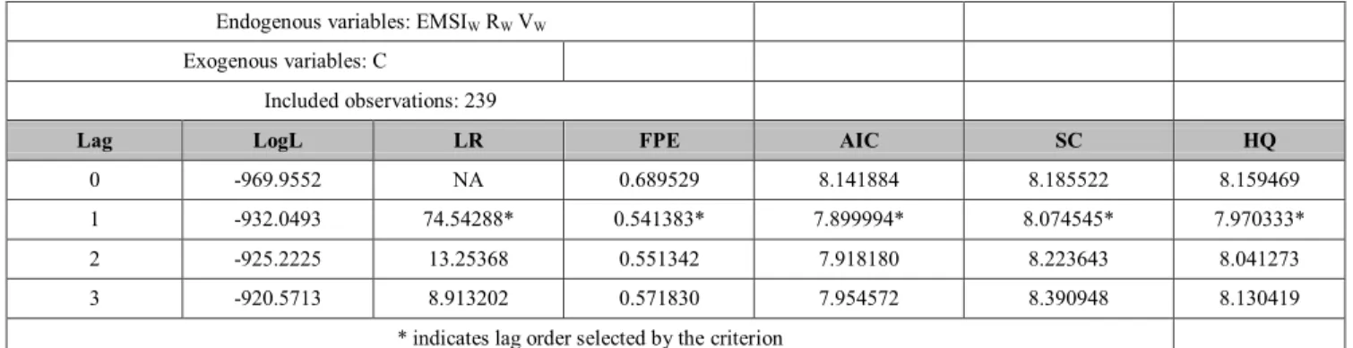
Sequential Modified Likelihood – Ratio test (LR), Final Prediction Error (FPE), Akaike Information Criterion (AIC), Schwarz Information Criterion (SC) and Hannan-Quinn Information Criterion (HQ). If there is any disagreement between these criteria, the lag order will be selected based on the Akaike Information Criterion (AIC). As can be seen from the Table 2, all information criteria choose one lag as the optimal lag order to be included in VAR model. It is expected that there is a causal relation between return with the lag of one week and current volume as well as current investor overconfidence
Table 13: Lag order selection in Vietnam stock market Endogenous variables: EMSIW RW VW
Exogenous variables: C
Included observations: 239
Lag LogL LR FPE AIC SC HQ
0 -969.9552 NA 0.689529 8.141884 8.185522 8.159469
1 -932.0493 74.54288* 0.541383* 7.899994* 8.074545* 7.970333*
2 -925.2225 13.25368 0.551342 7.918180 8.223643 8.041273
3 -920.5713 8.913202 0.571830 7.954572 8.390948 8.130419
* indicates lag order selected by the criterion
4.1.3. Granger Causality Test
The bivariate Granger causality test is performed with stock return, trading volume and Equity Market Sentiment Index – EMSI which is the proxy for confidence level of investors. The Table 3 demonstrates the test for causal relationship between these three variables.
Firstly, the null hypothesis that weekly stock returns do not Granger-cause weekly trading volume cannot be rejected at significant level of 5% as indicated by the p- value. Therefore, it is not possible to conclude that investors aggressively trade after making a profit with the lag order of one week. It is thus in disagreement with previous findings of (Odean, 1998) and (Gervais & Odean, 2001) about overconfidence hypothesis. The null hypothesis that trading volume Granger-cause stock returns cannot be rejected, either.
Secondly, the causal relationship between stock return and Equity Market Sentiment Index (EMSI) are tested.
According to the results in the Table 3, the null hypothesis that stock returns Granger-cause EMSI is rejected at significant level of 1%. It indicates that investor confidence can be driven by stock returns. It is likely that the more profitable the investment gets, the more confidence the investors have as they have more trust in their competency and the accuracy of information they hold. The exact sign of this relationship should be examined through the VAR model in the next section.
Thirdly, the causal relationship running from overconfidence proxy to market variables are not completely apparent. While the hypothesis that EMSI Granger-cause trading volume is rejected at significant level of 1%, the null hypothesis that EMSI does not
Granger-cause stock returns is accepted. This result suggests that overconfidence among Vietnamese investors affects the market volume but does not affect the market return at one lag period. It may indicate that Vietnam stock market is not completely efficient as investor overconfidence do drive the market to certain extent.
Table 14: Granger Causality Tests with lag 1
Null Hypothesis: Obs F-Statistic Prob.
RW does not Granger Cause EMSIW 246 9.37360 0.0024 EMSIW does not Granger Cause RW 0.31478 0.5753 VW does not Granger Cause EMSIW 246 38.7769 2.E-09 EMSIW does not Granger Cause VW 49.8150 2.E-11 VW does not Granger Cause RW 246 0.25903 0.6112 RW does not Granger Cause VW 1.05095 0.3063
4.1.4. The Vector Autoregressive Model (VAR)
As the Granger causality test suggests a causality link between variables, the VAR model depicts how variables correlate with each other at the optimal lag period.
Table 15: VAR model in Vietnam stock market
Equation: EMSIW = C(1)*EMSIW(-1) + C(2)*RW(-1) + C(3)*VW(-1) + C(4) Observations: 246
R-squared 0.183503 Mean dependent var -0.717246 Adjusted R-
squared 0.173381 S.D. dependent var 6.365784 S.E. of
regression 5.787681 Sum squared resid 8106.334 Durbin-Watson
stat 1.951494
Equation: RW = C(5)*EMSIW(-1) + C(6)*RW(-1) + C(7)*VW(-1) + C(8) Observations: 246
R-squared 0.002523 Mean dependent var -0.000874 Adjusted R-
squared -0.009843 S.D. dependent var 0.010849 S.E. of
regression 0.010902 Sum squared resid 0.028765 Durbin-Watson
stat 2.007282
Equation: VW = C(9)*EMSIW(-1) + C(10)*RW(-1) + C(11)*VW(-1) + C(12) Observations: 246
R-squared 0.190935 Mean dependent var -3.601367 Adjusted R-
squared 0.180906 S.D. dependent var 34.18077 S.E. of
regression 30.93491 Sum squared resid 231586.4 Durbin-Watson
stat 1.917192
The sign of the correlation coefficient indicates the direction in which these variables move. There are important points worth noting from the Table 4.
- The correlated coefficient between V_w and R_w (-1) is positive at 1% significant level, which shows the positive relationship between stock return and trading volume in Vietnam stock market. Although the causal relation between V_w and R_w (-1) is not proved in Granger causality test, V_w and R_w (-1) were found to move in the same direction, which is in agreement with previous studies.
- The coefficient between R_w (-1) and EMSI_w is positive, suggesting a positive relationship between investor confidence and one-lag stock return in Vietnam stock market at the significant level of 1%.
EMSI_w (-1) is positively correlated to V_w, which means that higher confidence level results in a higher trading volume with one lag period.
4.2. Testing Overconfidence in Singapore Stock Market
4.2.1. Stationarity Test on Time Series
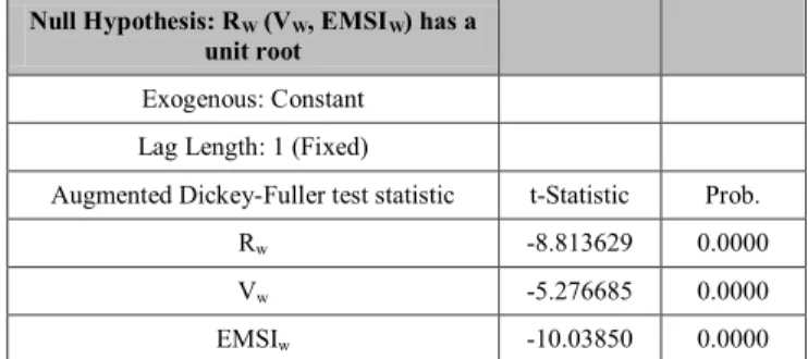
Applying similar process, the paper also use ADF test to examine whether all the time series variables of Singapore stock market are stationary. Because Augmented Dickey- Fuller test statistic is higher than critical values at all significance level of 1%, 5% and 10% in absolute term at 1%
significance level, the null hypothesis is rejected. It means that all variables including stock returns, trading volume and EMSI are stationary (see Table 5).
Table 16: Unit root test for 𝑅𝑤 𝑉𝑤 and 𝐸𝑀𝑆𝐼𝑤 in Singapore stock market
Null Hypothesis: RW (VW, EMSIW) has a unit root
Exogenous: Constant Lag Length: 1 (Fixed)
Augmented Dickey-Fuller test statistic t-Statistic Prob.
Rw -8.813629 0.0000
Vw -5.276685 0.0000
EMSIw -10.03850 0.0000
4.2.2. Lag Order Selection
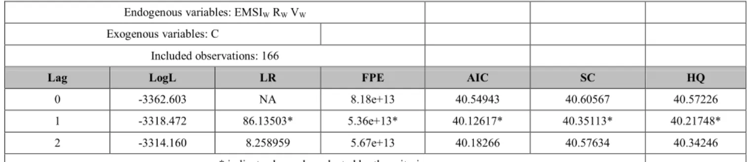
As can be seen from Table 6, the lag of one period is suggested by all information criteria. The principle of information criteria is to choose the lag order at which the value calculated by each criterion is minimum in order to ensure the stability of the model. Therefore, the lag of one period is chosen for testing hypothesis of overconfidence.
Table 17: Lag order selection in Singapore stock market Endogenous variables: EMSIW RW VW
Exogenous variables: C
Included observations: 166
Lag LogL LR FPE AIC SC HQ
0 -3362.603 NA 8.18e+13 40.54943 40.60567 40.57226
1 -3318.472 86.13503* 5.36e+13* 40.12617* 40.35113* 40.21748*
2 -3314.160 8.258959 5.67e+13 40.18266 40.57634 40.34246
* indicates lag order selected by the criterion
4.2.3. Granger Causality Test
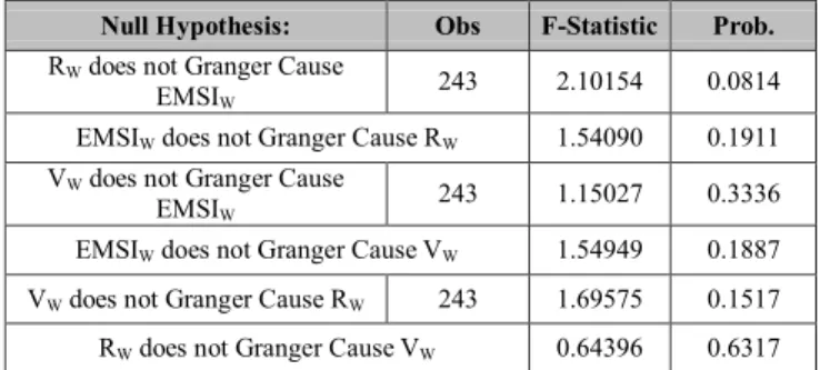
Results of the bivariate Granger causality test at 1 week lag is presented in Table 7:
Firstly, the null hypothesis that weekly stock returns do not Granger-cause weekly trading volume is rejected at 5%
significant level. Similar to Vietnamese investors, Singaporean investors eagerly raise their volume of transactions after seeing increase in returns. In the meantime, the null hypothesis that trading volume Granger- cause stock returns is also rejected at 1% significant level, suggesting potential negative impact of excessive trading volume on stock returns which should be further investigated in VAR model.
Next, the causal relationship between stock return and Equity Market Sentiment Index (EMSI) is tested.
Specifically, the null hypothesis that stock returns Granger- cause EMSI is rejected at significant level of 1%. It implies that increase in stock returns can contribute to investor overconfidence: If investors yield more returns, they become more confident thus irrationally increase their trading volume. Regarding impact of overconfidence on market variables, there is a causal relation running from EMSI_w (-1) to V_w because the null hypothesis that EMSI_w (-1) does not Granger-cause V_w is rejected at 5%
confidence level.
Table 18: Granger causality tests in Singapore with lag 1 Null Hypothesis: Obs F-Statistic Prob.
RW does not Granger Cause
EMSIW 173 19.0541 2.E-05
EMSIW does not Granger Cause RW 0.17653 0.6749 VW does not Granger Cause
EMSIW 173 0.42648 0.5146
EMSIW does not Granger Cause VW 6.47553 0.0118 VW does not Granger Cause RW 173 8.81665 0.0034 RW does not Granger Cause VW 3.96176 0.0481
4.2.4. The Vector Autoregressive Model (VAR)
To analyse the trend of the mutual impact among three
variables, the authors estimate the coefficients of OLS regression on VAR model. In terms of stock returns and trading volume, it is essential to look into the relation between trading volume and lagged stock returns, and the relation between stock returns and lagged trading volume.
In the former test, there is a positive relationship between these variables at 5% significant level, which means that one-lag stock returns are positively correlated with trading volume. Whereas, in the latter test, a negative relation between lagged trading volume and stock returns is found, which means that excessive trading volume will harm the subsequent returns.
Table 19: VAR model in Singapore stock market
Equation: EMSIW = C(1)*EMSIW(-1) + C(2)*RW(-1) + C(3)*VW(-1) + C(4) Observations: 173
R-squared 0.107488 Mean dependent var -2.324152 Adjusted R-squared 0.091644 S.D. dependent var 5.434722 S.E. of regression 5.179709 Sum squared resid 4534.167 Durbin-Watson stat 1.923283
Equation: RW = C(5)*EMSIW(-1) + C(6)*RW(-1) + C(7)*VW(-1) + C(8) Observations: 173
R-squared 0.065039 Mean dependent var -0.000170 Adjusted R-squared 0.048442 S.D. dependent var 0.006443 S.E. of regression 0.006285 Sum squared resid 0.006677 Durbin-Watson stat 2.062718
Equation: VW = C(9)*EMSIW(-1) + C(10)*RW(-1) + C(11)*VW(-1) + C(12) Observations: 173
R-squared 0.307808 Mean dependent var 1.15E+09 Adjusted R-squared 0.295521 S.D. dependent var 2.73E+08 S.E. of regression 2.29E+08 Sum squared resid 8.90E+18 Durbin-Watson stat 2.174367
For the relation between overconfidence and market variables (return, volume), the VAR model shows that