Next:Linear Algebraic and EquationsUp:Numerical Analysis for ChemicalPrevious:Modeling, Computers, and Error Subsections
z Backeting Methods
{ Graphical Methods
{ The Bisection Method
{ The False-Position Method
z Open Methods
{ Simple Fixed-point Iteration
{ The Newton-Raphson Method
{ The Secant Method
{ Multiple Roots
{ Systems of Nonlinear Equations
z Roots of Polynomials
{ Polynomials in Engineering and Science
{ Computing with Polynomials
{ Conventional Methods
{ Root Location with Libraries and Packages
z Engineering Applications: Roots of Equations
Roots of Equations Backeting Methods
Graphical Methods
A simple method for obtaining an estimate of the root of the equation is to make a plot of the function and observe where it crosses the x axis.
The Bisection Method
In general, if and
then there is at least one real root between .
The False-Position Method
A shortcoming of the bisection method
z equally dividing the interval
z no account for for the magnitudes of and
(2.1)
An alternative method is to join and
improved estimate of the root. This mothod is called as method of false position, regula falsi, or linear interpolation method.
The false-position formula is
See Figure 5.14 in textbook
Open Methods
z bracketing method : the root is located within an interval prescribed by a lower and an upper bound.
z open method : require only a single starting value of x or two starting point that do not necessarily bracket the root.
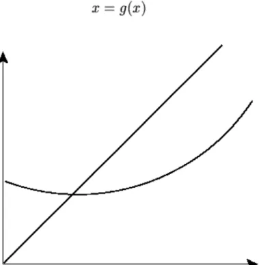
Simple Fixed-point Iteration
-point iteration by rearranging the
function -hand side of the equation:
The Newton-Raphson Method
If the initial guess at the root is , a tangent can be extended from the point . The point where this tangent crosses the x axis usaually represents an improved estimate of the root.
The Newton-Raphson formula is
(2.2)
(2.3)
Figure 2.1: Graphical depiction of simple fixed-point method.
Pitfalls of the Newton-Raphson Method are shown in Figure 6.6
The Secant Method
A potential problem in implementing the Newton-Raphson method is the evaluation of the derivative. In Secant method the derivative is approximated by a backward finite divided difference
The Secant formula is
The difference between the secant method and the false-position method is how one of the initial values is replaced by the new estimate.
Rather than using two arbitrary values to estimate the derivative, an alternative approach involves a fractional perturbation of the independent variable to estimate ,
where is a small perturbation fraction. This approximation gives the following iterative equation:
Multiple Roots
Some difficulities in multiple roots problem
z no change in sign at even multiple roots
z go to zero at the root
z the Newton-Raphson method and secant method show linear, rather than quadratic, convergence for multiple roots.
Another alternative is to define a new function ,
(2.4)
(2.5)
(2.6)
(2.7)
(2.8)
An alternative form of the Newton-Raphson method:
where is
And finally
Systems of Nonlinear Equations
The Newton-Raphson method can be used to solve a set of nonlinear equations. The Newton-Raphson method employ the derivative of a function to estimate its intercept with the axis of the independent variable. This estimate was based on a first-order Taylor series expansion. For example, we consider two variable case,
A first-order Taylor series expasion can be written as
The above equation can be rearranged to give
(2.9)
(2.10)
(2.11)
(2.12)
(2.13)
(2.14)
(2.15)
(2.16)
(2.17)
(2.18)
Finally
Roots of Polynomials
The roots of polynomials have the following properties
z For an nth-order equation, there are n real and complex roots.
z If n is odd, there is at least one real root.
z If complex roots exist, they exist in conjugate pairs.
Polynomials in Engineering and Science
Polynomial are used extensively in curve-fitting. However, another most important application is in characterizing dynamic system and, in particular, linear systems.
For example, we consider the following simple second-order ordinary differential equation:
where is the forcing function. And the above ODE can be expressed as a system of 2 first-order ODEs by defining a new variable z,
This reduces the problem to solving
(2.19)
(2.20)
(2.21)
(2.22)
(2.23)
(2.24)
In a simliar fashion, nth-order linear ODE can always be expressed as a system of n first-order ODEs.
The general solution of ODE equation deals with the case when the forcing function is set to zero.
This equation gives something very fundamental about the system being simulated-that is, how the system reponds in the absence of external stimuli. The general solution to all unforced linear system is of the form .
or cancelling the exponential terms,
This polynomial is called as characteristic equation and these r's are referred to as eigenvalues.
z overdamped case : all real roots
z critically damped case : only one root
z underdamped case : all complex roots
Computing with Polynomials
For nth-order polynomial calculation, general approach requires
use a nested format, additions are required.
DO j=n, 0
p = p * x + a(j) END DO
If you want to find all roots of a polynomial, you have to remove the found root before another processing. This removal process is referred to as polynomial deflation.
Conventional Methods
z Müller's method : projects a parabola through three points.
z Bairstow's method:
1. guess a value for the root
2. divide the polynomial by the factor
3. determine whether there is a reminder. If not, the guess is was perfect and the root is equal to. If there is a reminder, the guess can be systematically adjusted and the procedure repeated until the reminder disappears.
(2.25)
(2.26)
(2.27)
(2.28)
Root Location with Libraries and Packages
z Matlab:
{ roots
{ poly
{ polyval
{ residue
{ conv
{ deconv
z IMSL:
{ ZREAL
Engineering Applications: Roots of Equations
See the textbook
Next:Linear Algebraic and EquationsUp:Numerical Analysis for ChemicalPrevious:Modeling, Computers, and Error Taechul Lee
2001-11-29