Multivariate EWMA control charts for monitoring the variance-covariance matrix

Multivariate EWMA control charts for monitoring the variance-covariance matrix

Jeong-Im Jeong ¹ · Gyo-Young Cho ²

12 Department of Statistics, Kyungpook National University

Received 14 May 2012, revised 31 May 2012, accepted 5 June 2012

Abstract

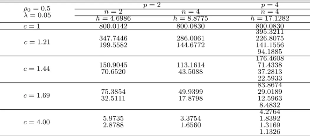
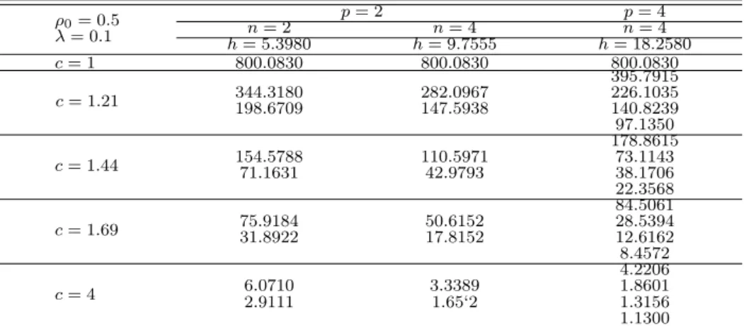
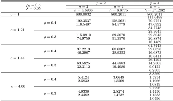
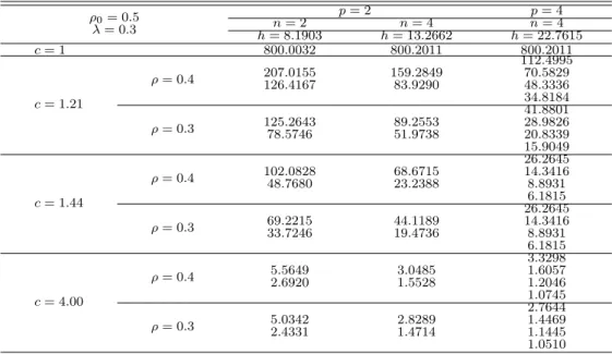
We know that the exponentially weighted moving average (EWMA) control charts are sensitive to detecting relatively small shifts. Multivariate EWMA control charts are considered for monitoring of variance-covariance matrix when the distribution of process variables is multivariate normal. The performances of the proposed EWMA control charts are evaluated in term of average run length (ARL). The performance is investigated in three types of shifts in the variance-covariance matrix, that is, the vari- ances, covariances, and variances and covariances are changed respectively. Numerical results show that all multivariate EWMA control charts considered in this paper are effective in detecting several kinds of shifts in the variance-covariance matrix.

Keywords: Average run length, multivariate exponentially weighted moving average control chart, variance-covariance matrix.

1. Introduction

A control chart is very useful in monitoring various production processes. There are many situations in which the simultaneous control of two or more related quality characteristics is necessary. To monitor the product quality in the multivariate production processes, it is more advantageous to use multivariate control charts rather than univariate control charts.

Multivariate control charts have been interested in new research and remain an important area of research in statistical quality control.

Control charts are continuously monitoring the production process to detect quickly the changes that may produce any deterioration in the quality of the product. Control charts are becoming increasingly common for the quality of processes to be characterized by multiple variables.

The multivariate control charts of the Shewhart type was introduced by Hotelling (1947).

This multivariate Shewhart chart was constructed based on Hotelling’s T ² statistic. Jackson (1959), and Ghare and Torgersen (1968) presented a multivariate Shewhart chart based on Hotelling’s T ² statistic. Other multivariate Shewhart charts are discussed by Alt (1984), Wierda (1994), and Lowry and Montgomery (1995).

1

Ph. D. student, Department of Statistics, Kyungpook National University, Daegu 702-701, Korea.

2

Corresponding author: Professor, Department of Statistics, Kyungpook National University, Daegu

702-701, Korea. E-mail: [email protected]

The exponentially weighted moving average (EWMA) control chart was introduced by Roberts (1959). It is well known that the EWMA control charts are much more effective than Shewhart-type charts for detecting small and moderate shifts in process parameters.

The EWMA charts have been developed to detect shifts in the process variability (Hunter, 1968; Robinson and Ho, 1978; Crowder, 1987, 1989; Lucas and Saccucci, 1990; Saccucci and Lucas, 1990). Sweet (1986) suggest using two EWMA control charts, one for detecting mean shifts and the other for detecting shifts of variances. MacGregor and Harris (1993) propose EWMA control charts for controlling vairance that also could be used for individual observations.

The development of multivariate EWMA control charts has concentrated on the problem of monitoring mean vector µ. A multivariate extension of the univariate control chart was studied by Lowry et al. (1992), Prabhu and Runger (1997), Reynolds and Kim (2005), and Lim and Cho (2008), Chang and Shin (2009), Cho (2010), and Im and Cho (2009). We study the multivariate EWMA control charts for monitoring the variance-covariance matrix Σ.

2. Notation and assumptions

In working with the multivariate normal distribution, it will be convenient to let σ rep- resent the vector of standard deviations of the p variables. Let µ ₀ , Σ ₀ , and σ ₀ represent the in-control values for µ, Σ, and σ, respectively. In practice, some of the in-control parameter values would need to be estimated during a Phase I period when process data are collected for purposes of parameter estimation. Here we consider control chart performance in Phase II under the simplifying assumption that the in-control parameter values are known.

Suppose that the process will be monitored by taking a sample of n ≥ p independent observation vectors at each sampling point, where the sampling points are d time units apart. Let X kij represent observation j (j = 1, 2, · · · , n) for variable i (i = 1, 2, · · · , p) at sampling point k (k = 1, 2, · · · ), and let the corresponding standardized observation be

Z kij = (X kij − µ 0i )/σ 0i ,

where µ 0i is the ith component of target mean vector µ 0 , and σ 0i is the ith diagonal com- ponent of σ 0 . Also let

Z _kj = (Z _k1j , Z _k2j , · · · , Z _kpj )

, j = 1, 2, · · · , n.

be the vector of standardized observations for observation vector j at sampling point k.

Let Σ _Z be the covariance matrix of Z _kj , and let Σ _Z0 be the in-control value of Σ _Z . The in-control distribution of Z _kij is standard normal, so Σ _Z0 is also the in-control correlation matrix of the unstandardized observations.

When n ≥ p, some control statistics used for monitoring Σ are functions of the sample estimates Σ Z . At sampling point k, let b Σ Zk be the maximum likelihood estimator of Σ Z , where the (i, i

) element of b Σ Zk is P n

j=1 Z kij Z _ki

_j /n.

We investigate a number of different control charts based on plotting multivariate EWMA

control statistics.

3. Multivariate EWMA control charts

Hotelling (1947) proposed a Shewhart-type control chart for Σ using the statistic Y k given by (3.1).

n

X

j=1

(Z k1j , Z k2j, · · · , Z kpj )Σ ⁻¹ _Z0 (Z k1j , Z k2j , · · · , Z kpj ) ⁰ (3.1)

= ntr(b Σ _Zk Σ ⁻¹ _Z0 ) = Y _k

where Σ ₀ is assumed to be known. When the process is in control, the distribution of the control statistic Y _k is chi-square with np degrees of freedom.

For constructing multivariate EWMA control charts for monitoring the variance-covariance matrix, we use the statistic Y k given by (3.1). A multivariate EWMA control chart for mon- itoring Σ is based on the statistic

E k = (1 − λ)E k−1 + λY k , k = 1, 2, · · · (3.2) where E 0 = 0 and λ is weighting or tuning parameter satisfying 0 < λ ≤ 1.

Therefore, a multivariate EWMA based on the statistic E k signals whenever

E k ≥ h, (3.3)

where a control limit h can be obtained to satisfy a specified in-control ARL. We can use a Markov chain approach, integral equations or simulations to get h value. If the process shifts from Σ ₀ , then it is necessary to use simulations to get ARL values.

4. Numerical performances and concluding remarks

In this section the following control procedures are compared on the basis of their ARL performances of the Multivariate EWMA control charts with control statistic given by (3.2).

The performance of the control charts for monitoring the variance-covariance matrix depends on the value of Σ. The following types of shifts were considered :

(1) variances are changed and covariances are not changed, (2) covariances are changed and variances are not changed, (3) variances and covariances are simultaneously changed.

The ARL and h values in the multivariate EWMA control chart based on (3.2) were obtained by using 10,000 runs. Tables 4.1-4.9 give the h and ARL values for p = 2, 4, ρ 0 = 0.5, and λ = 0.05, 0.1, 0.3. The ARL at Σ = Σ 0 is approximately 800. The parameters h were obtained to give specified ARL when the process is in control.

When variances are changed, the values in the Tables 4.1-4.3 are h and ARL for λ = 0.05, 0.1, 0.3, respectively. The numbers in each cell from the row named c = 1.21 to the row named c = 4.00 in Tables 4.1-4.3 are ARLs when one, two,..., p variances are changed re- spectively. Standard deviations are changed from σ ₀ to σ = √

cσ ₀ , for c = 1.21, 1.44, 1.69, 4.

As shown in Tables 4.1-4.3, the multivariate EWMA control charts given by (3.2) for moni- toring the variance-covariance matrix are effective in detecting only changes of variances in Σ.

When covariances are changed, the values in the Tables 4.4-4.6 are h and ARL for λ = 0.05, 0.1, 0.3, respectively. Covariances are changed from ρ 0 = 0.5 to ρ = 0.45, 0.35, 0.25, 0.15, 0.05. As shown in Tables 4.4-4.6, the multivariate EWMA control charts given by (3.2) for monitoring the variance-covariance matrix are effective in detecting only changes of covariances in Σ.

When variances and covariances are simultaneously changed, the values in the Tables 4.7- 4.9 are h and ARL for λ = 0.05, 0.1, 0.3, respectively. The numbers in each cell from the row named c = 1.21 to the row named c = 4.00 in Tables 4.7-4.8 are ARLs when one, two,..., p variances and p covariances are simultaneously changed respectively. As shown in Tables 4.7-4.9, the multivariate EWMA control charts given by (3.2) for monitoring the variance- covariance matrix are also effective in detecting simultaneously changes of variances and covariances in Σ.

Tables 4.1-4.9 show that all multivariate EWMA control charts considered in this paper are effective in detecting several kinds of shifts in the variance-covariance matrix. But in the Tables 4.1-4.9, the ARL values are not much different for λ = 0.05, 0.1, 0.3.

Table 4.1 ARL for multivariate EWMA control charts when variances are changed (λ = 0.05)

ρ

= 0.5 p = 2 p = 4

λ = 0.05 n = 2 n = 4 n = 4

h = 4.6986 h = 8.8775 h = 17.1282

c = 1 800.0142 800.0830 800.0830

c = 1.21

395.3211

347.7446 286.0061 226.8075

199.5582 144.6772 141.1556

94.1885

c = 1.44

176.4608

150.9045 113.1614 71.4338

70.6520 43.5088 37.2813

22.5933

c = 1.69

83.8674

75.3854 49.9399 29.0189

32.5111 17.8798 12.5963

8.4832

c = 4.00

4.2764

5.9735 3.3754 1.8392

2.8788 1.6560 1.3169

1.1326

Table 4.2 ARL for multivariate EWMA control charts when variances are changed (λ = 0.1)

ρ

= 0.5 p = 2 p = 4

λ = 0.1 n = 2 n = 4 n = 4

h = 5.3980 h = 9.7555 h = 18.2580

c = 1 800.0830 800.0830 800.0830

c = 1.21

395.7915

344.3180 282.0967 226.1035

198.6709 147.5938 140.8239

97.1350

c = 1.44

178.8615

154.5788 110.5971 73.1143

71.1631 42.9793 38.1706

22.3568

c = 1.69

84.5061

75.9184 50.6152 28.5394

31.8922 17.8152 12.6162

8.4572

c = 4

4.2206

6.0710 3.3389 1.8601

2.9111 1.65‘2 1.3156

1.1300

Table 4.3 ARL for multivariate EWMA control charts when variances are changed (λ = 0.3)

ρ

= 0.5 p = 2 p = 4

λ = 0.3 n = 2 n = 4 n = 4

h = 8.1903 h = 13.2662 h = 22.7615

c = 1 800.0830 800.0830 800.0830

c = 1.21

392.5439

339.7663 291.7363 224.0184

198.8770 145.5450 140.7379

96.0928

c = 1.44

179.7888

152.9800 111.3255 71.9902

71.0416 43.4007 37.9122

22.8305

c = 1.69

83.5025

75.9006 50.4200 28.4059

32.4269 17.5431 12.2888

8.4714

c = 4.00

4.2671

6.0403 3.3626 1.8471

2.9246 1.6549 1.3122

1.1239

Table 4.4 ARL for multivariate EWMA control charts when covariances are changed (λ = 0.05)

ρ

= 0.5 p = 2 p = 4

λ = 0.05 n = 2 n = 4 n = 4

h = 4.6986 h = 8.8775 h = 17.1282

ρ = 0.5 800.0142 799.9887 800.1258

ρ = 0.45 589.9066 566.4876 377.0370

ρ = 0.35 316.6366 279.2700 110.4036

ρ = 0.25 176.6587 138.9008 42.7011

ρ = 0.15 108.1872 71.2605 20.9380

ρ = 0.05 72.6904 50.4704 12.0682

Table 4.5 ARL for multivariate EWMA controls chart when covariances are changed (λ = 0.1)

ρ

= 0.5 p = 2 p = 4

λ = 0.1 n = 2 n = 4 n = 4

h = 5.3980 h = 9.7555 h = 17.1282

ρ = 0.5 799.9645 799.9020 800.0820

ρ = 0.45 598.1236 565.7006 382.9879

ρ = 0.35 313.3510 274.7477 109.2216

ρ = 0.25 180.4640 142.7244 43.2916

ρ = 0.15 108.8055 81.1860 21.0628

ρ = 0.05 71.8636 50.4704 12.3642

Table 4.6 ARL for multivariate EWMA control charts when covariances are changed (λ = 0.3)

ρ

= 0.5 p = 2 p = 4

λ = 0.3 n = 2 n = 4 n = 4

h = 8.1903 h = 13.2662 h = 22.7615

ρ = 0.5 799.9889 799.9158 800.1380

ρ = 0.45 590.9664 560.3408 377.1021

ρ = 0.35 317.9438 273.9652 109.2003

ρ = 0.25 182.4872 140.1832 42.2236

ρ = 0.15 107.7375 79.4267 20.8749

ρ = 0.05 71.2405 50.1246 11.9735

Table 4.7 ARL for multivariate EWMA control charts when variances and covariances are changed (λ = 0.05)

ρ

= 0.5 p = 2 p = 4

λ = 0.05 n = 2 n = 4 n = 4

h = 4.6986 h = 8.8775 h = 17.1282

c = 1 800.0032 800.2011 800.2011

c = 1.21

ρ = 0.4

111.6488

192.3537 158.5621 70.2721

116.5407 84.5779 47.6992

34.7748

ρ = 0.3

29.3045

115.0910 89.5070 29.3045

74.9759 51.3570 20.8874

16.1489

c = 1.44

ρ = 0.4

61.7443

97.2219 68.6802 29.0628

46.2967 28.9353 16.6873

10.8411

ρ = 0.3

26.1292

63.5825 44.5883 14.2505

32.3112 19.4080 9.0122

6.2505

c = 4.00

ρ = 0.4

3.3569

5.4124 3.0649 1.5954

2.5832 1.5509 1.1966

1.0819

ρ = 0.3

2.7296

4.9336 2.8274 1.4450

2.4482 1.4732 1.1533

1.0496

Table 4.8 ARL for multivariate EWMA control charts when variances and covariances are changed (λ = 0.1)

ρ

= 0.5 p = 2 p = 4

λ = 0.1 n = 2 n = 4 n = 4

h = 5.3980 h = 9.7555 h = 18.2580

c = 1 800.0032 800.2011 800.2011

c = 1.21

ρ = 0.4

110.6742

206.0894 162.0527 70.9878

124.8640 85.7969 48.5659

35.2827

ρ = 0.3

42.5713

124.8409 89.2529 28.7698

78.4954 51.7762 21.4159

16.0013

c = 1.44

ρ = 0.4

62.2538

103.8395 69.0140 29.1244

48.9727 28.8839 16.7269

10.6993

ρ = 0.3

26.8357

68.1848 43.3188 14.4030

34.4964 19.5606 8.9106

6.2212

c = 4.00

ρ = 0.4

3.3860

5.4911 3.0632 1.6314

2.6538 1.5453 1.2070

1.0785

ρ = 0.3

2.7121

5.0974 2.7951 1.4393

2.4886 1.4800 1.1426

1.0527

Table 4.9 ARL for multivariate EWMA control charts when variances and covariances are changed (λ = 0.3)

ρ

= 0.5 p = 2 p = 4

λ = 0.3 n = 2 n = 4 n = 4

h = 8.1903 h = 13.2662 h = 22.7615

c = 1 800.0032 800.2011 800.2011

c = 1.21

ρ = 0.4

112.4995

207.0155 159.2849 70.5829

126.4167 83.9290 48.3336

34.8184

ρ = 0.3

41.8801

125.2643 89.2553 28.9826

78.5746 51.9738 20.8339

15.9049

c = 1.44

ρ = 0.4

26.2645

102.0828 68.6715 14.3416

48.7680 23.2388 8.8931

6.1815

ρ = 0.3

26.2645

69.2215 44.1189 14.3416

33.7246 19.4736 8.8931

6.1815

c = 4.00

ρ = 0.4

3.3298

5.5649 3.0485 1.6057

2.6920 1.5528 1.2046

1.0745

ρ = 0.3

2.7644

5.0342 2.8289 1.4469

2.4331 1.4714 1.1445

1.0510

References

Alt, F. B. (1984). Multivariate control charts. In Encyclopedia of Statistical Sciences, edited by S. Kotz and N. L. Johnson, John Wiley, New York.

Chang, D. J. and Shin, J. K. (2009). Variable sampling interval control charts for variance-covariance matrix.

Journal of the Korean Data & Information Science Society, 21, 999-1008.

Cho, G. Y. (2010). Multivariate Shewhart control charts with variable sampling intervals. Journal of the Korean Data & Information Science Society, 21, 999-1008.

Crowder, S. V (1987). A simple method for studying run length distributions of exponentially weighted moving average control charts. Technometircs, 29, 401-407.

Crowder, S. V (1989). Design of exponentially weighted moving average schemes. Journal of Quality Tech- nology, 21, 155-162.

Ghare, P. H. and Torgerson, P. E. (1968). The multicharacteristic control chart. Journal of Industrial Engineering, 19, 269-272.

Hotelling, H. (1947). Multivariate quality control, techniques of statistical analysis, McGraw-Hill, New York, 111-184.

Hunter, J. S. (1968). The exponentially weighted moving average. Journal of Quality Technology, 18, 203- 210.

Im, C. D. and Cho, G. Y. (2009). Multiparameter CUSUM charts with variable sampling intervals. Journal of the Korean Data & Information Science Society, 20, 593-599.

Jackson, J. S. (1959). Quality control methods for several related variables. Technometrics, 1, 359-377.

Lim, C and Cho, G. Y. (2008). A new EWMA control chart for monitoring the covariance matrix of bivariate processes. Journal of the Korean Data & Information Science Society, 19, 677-683.

Lowry, C. A. and Montgomery, D. C. (1995). A review of multivariate control charts. IIE Transactions, 27, 800-810.

Lowry, C. A., Woodall, W. H., Champ, C. W. and Rigdon, S. E. (1992). A multivariate exponentially weighted moving average control chart. Technometrics, 34, 46-53.

Lucas, J. M. and Saccucci, M. S. (1990). Exponentially weighted moving average control schemes: Properties and enhancements. Technometrics, 32, 1-12.

MacGregor, J. F. and Jarris, T. J. (1993). The exponentially weighted moving variance. Journal of Quality Technology, 25, 106-118.

Reynolds, M. R., Jr. and Kim, G. (2005). Multivariate monitoring of the mean vector using sequential sampling. Journal of Quality Technology, 37, 149-162.

Roberts, S. W. (1959). Control chart tests based on geometric moving averages. Technometrics, 1, 239-250.

Robinson, P. B. and Ho, T. Y. (1978). Average run length of geometric moving average charts by numerical methods. Technometrics, 20, 85-93.

Prabhu, S. S. and Runger, G. C. (1997). Designing a multivariate EWMA control chart. Journal of Quality Technology, 29, 8-15.

Saccucci, M. S. and Lucas, J. M. (1990). Average run lengths for exponentially weighted moving average control schemes using the Markov chain approach. Jounal of Quality Technology, 22, 154-162.

Sweet, A. L. (1986). Control chart using coupled exponentially weighted moving averages. IIE Transactions 18, 26-33.

Wierda, S. J. (1994). multivariate statistical process control - recent results and directions for future research.

Statistica Neerlandica, 48, 147-168.