Multivariate Shewhart control charts for monitoring the variance-covariance matrix

Multivariate Shewhart control charts for monitoring the variance-covariance matrix ^†

Jeong-Im Jeong ¹ · Gyo-Young Cho ²

12 Department of Statistics, Kyungpook National University

Received 29 April 2012, revised 17 May 2012, accepted 22 May 2012

Abstract

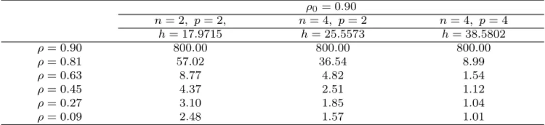
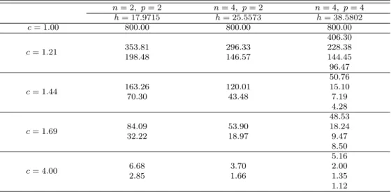
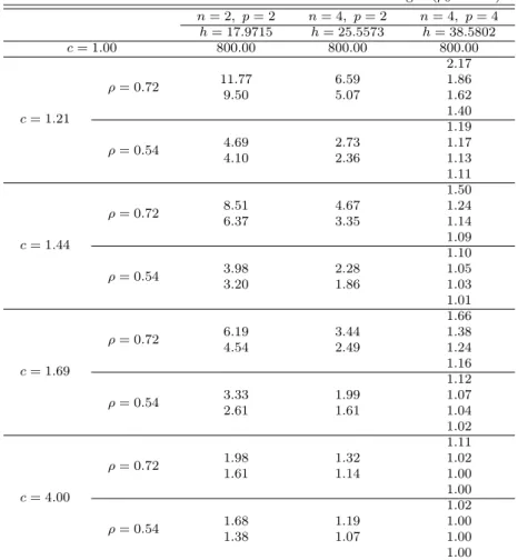
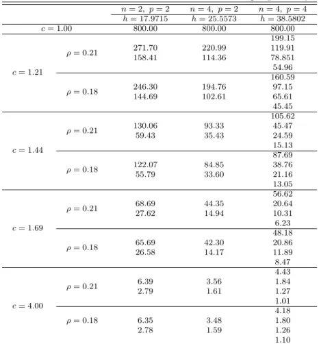
Multivariate Shewhart control charts are considered for the simultaneous moni- toring the variance-covariance matrix when the joint distribution of process variables is multivariate normal. The performances of the multivariate Shewhart control charts based on control statistic proposed by Hotelling (1947) are evaluated in term of average run length (ARL) for 2 or 4 correlated variables, 2 or 4 samples at each sampling point.

The performance is investigated in three cases, that is, the variances, covariances, and variances and covariances are changed respectively.

Keywords: Average run length, multivariate Shewhart control chart, variance-covariance matrix.

1. Introduction

Control charts are the simplest type of statistical process-control procedure. Control chart are used to detect changes in the parameters of the distribution of these variables. Control charts are continuously monitoring the production process to detect quickly the changes which is producing any deterioration in the quality of the product. Im and Cho (2009) stud- ied simultaneously monitoring the mean and variance in the production processes. There are many situations in which the simultaneous control of two or more related quality characteris- tics is necessary. There are various approaches to constructing control charts for multivarite data. The original work in multivariate control charts was introduced by Hotelling (1947) which is the multivariate Shewhart chart based on Hotelling’s T ² statistic. Jackson (1959), and Ghare and Torgersen (1968) presented multivariate Shewhart control charts based on Hotelling’s T ² statistic. Other multivariate Shewhart control charts are discussed by Alt (1984), Wierda (1994), and Lowry and Montgomery (1995). Exponentially weighted moving average (EWMA) charts are much more effective than Shewhart-type charts for detecting small and moderate shifts in process parameters. The development of multivariate EWMA control charts has concentrated on the problem of monitoring mean vector. A multivariate extension of the EWMA chart was proposed by Lowry et al. (1992), Prabhu and Runger

† This research was supported by Kyungpook National University Research Fund, 2011.

1

Ph. D. student, Department of Statistics, Kyungpook National University, Daegu 702-701, Korea.

2

Corresponding author: Professor, Department of Statistics, Kyungpook National University, Daegu

702-701, Korea. E-mail: [email protected]

(1997), Reynolds and Kim (2005), and Reynolds and Cho (2006). The multivariate control charts for monitoring variance-covariance matrix were studied by Chang and Shin (2009), Lim and Cho (2010), Na et al. (2010). In this paper we study multivariate Shewhart control charts using the function of the maximum likelihood estimator for monitoring the variance- covariance matrix

2. Notations and assumptions

The multivariate normal distribution of the observation will be convenient to let σ repre- sent the vector of standard deviations of the variables. Let µ 0 , Σ 0 and σ 0 be the in-control values of µ, Σ and σ. In practice, some of the in-control parameter values would need to be estimated during a Phase Ⅰ period when process data are collected for purposes of parame- ter estimation. Here we consider control chart performance in Phase Ⅱ under the simplifying assumption that the in-control parameter values are known. Considering this case of known in-control parameter values is sufficient to evaluate the relative performance of the different control chart. We will usually refer to µ 0 as the target, even though, in practice, some of the components of µ 0 may correspond to estimated means rather than to specified target values.

Suppose that the process will be monitored by taking a sample of n ≥ 1 independent observation vectors at each sampling point, where the sampling points are d time units apart. Let X _kij be the jth observation for variable i at sampling point k for k = 1, 2, · · · , i = 1, 2, · · · , p and j = 1, 2, · · · , n, and let the corresponding standardized observation be

Z kij = (X kij − µ 0i )/σ 0i ,

where µ _0i is the ith component of µ ₀ and σ _0i is the ith component of σ ₀ . Also let Z kj = (Z k1j , Z k2j , · · · , Z kpj )

, j = 1, 2, · · · , n

be the vector of standardized observations for observation vector j at sampling point k.

Let Σ Z be the covariance matrix of Z kj , and let Σ Z0 be the in-control value of Σ Z . The in-control distribution of Z kij is standard normal, so Σ Z0 is also the in-control correlation matrix of the unstandardized observations.

Let X _ki = P n

j=1 X _kij /n be the sample mean for variable i at sampling point k, and define the standardized sample mean to be

Z ki = √

n(X ki − µ 0i )/σ 0i , i = 1, 2, · · · , p.

When n ≥ p, some control statistics used for monitoring Σ are functions of the sample estimates Σ _Z . At sampling point k, let b Σ _Zk be the maximum likelihood estimator of Σ _Z , where the (i, i

) element of b Σ _Zk is P n

j=1 Z _kij Z _ki

_j /n.

We investigate a number of control charts based on plotting Shewharts control statistics.

3. Multivariate Shewhart control charts

The Shewhart control chart is one of the most widely used control charts for monitoring

the parameters of a process. Shewhart control charts are very sensitive to the choice of

the sample size (Reynolds and Stoumbos, 2004a, 2004b). Shewhart control chart is used to display sample data from a process for the purpose of determining whether a production process is in-control, for bringing an out-of-control process into in-control, and for monitoring a process to make sure that it stays in-control. A Shewhart control chart has good ability to detect large changes in monitored parameter quickly. The basic Shewhart control chart, although simple to understand and apply, uses only the information in the current sample and is thus relatively inefficient in detect small shifts in control parameter.

At sampling point, multivariate control charts for monitoring the variance-covariance ma- trix can be constructed by using the statistic for testing H 0 : Σ = Σ 0 vs H 1 : Σ 6= Σ 0 .

The Shewhart-type control chart proposed by Hotelling (1947) for monitoring mean vector (frequently called Hotelling’s T ² chart) was originally developed for the case in which Σ 0

is unknown. See Mason and Young (2002) for a thorough discussion of the application of this control chart. If Σ ₀ is assumed to be known, then this control chart is equivalent to a control chart based on the statistic

(Z _k1 , Z _k2 , · · · , Z _kp )Σ ⁻¹ _Z0 (Z _k1 , Z _k2 , · · · , Z _kp ) ⁰ (3.1) used with an upper control limit (UCL).

Hotelling (1947) proposed a control chart for monitoring Σ based on

n

X

j=1

(Z k1j , Z k2j, · · · , Z kpj )Σ ⁻¹ _Z0 (Z k1j , Z k2j , · · · , Z kpj ) ⁰ = ntr(b Σ Zk Σ ⁻¹ _Z0 ) = Y k . (3.2)

This control chart has both a lower control limit (LCL) and an UCL. When the process is in control, the distribution of the control statistic is chi-squred with degrees of freedom.

For a Shewhart control chart, control limits based on the statistic Y k would be set by using percentage point of Y _k , and signals whenever

Y _k ≥ h (3.3)

where h can be obtained to satisfy a specified in-control ARL.

If the process shifts from Σ ₀ then it is difficult to obtain the exact distribution of Y _k . Thus in order to obtain the percentage points of Y k when the process is in out-of-control state, it is necessary to use simulations.

But, this control chart has both a LCL and an UCL. For some additional discussion of Shewhart charts for monitoring Σ, see Alt (1984), Lowry and Montgomery (1995), and Tang and Barnett (1996a, 1996b).

4. Numerical performances and concluding remarks

The ability of a control chart to detect any shifts in the production process is determined by the length of time required to signal. Thus, a good control chart detect shifts quickly in the process when the process is out-of-control state, and produce few false alarms when the process is in-control state.

The performance of the control charts considered in this paper are evaluated on the basis

of their average run length performance. The ARL values for the multivarte control chart

using equation (3.2) when the process is in control can be obtained by using chi-squared distribution. ARL values for various shifts were calculated by using 10,000 replications.

In order to evaluate the performances and compare the proposed multivariate Shewharts fairly, it is necessary to calibrate each control chart so that on-target ARL be the same for all proposed control charts. In our computation, each control chart was calibrated so that the on-target ARL was approximately equal to 800.0 and the sample size for each control chart was 2 and 4 for p = 2 and p = 4. The performance of the charts for monitoring the variance-covariance matrix depends on the value of Σ. The following types of shifts were considered :

(1) variances are changed and covariances are not changed, (2) covariances are changed and variances are not changed, (3) variances and covariances are simultaneously changed.

Tables 4.1-4.3 give the values of and ARL values for n = 2, 4 and p = 2, 4 and three different in-control correlation coefficients ρ ₀ = 0.9, 0.5, 0.3 when covariances are changed and variances are not changed. Here the changed values of considered in Tables 4.1-4.3 are those of decreased by 10%, 30%, 50%, 70% and 90% of ρ ₀ values, respectively. As shown in Tables 4.1-4.3, the multivariate Shewhart control charts proposed by Hotelling (1947) for monitoring the variance-covariance matrix are effective in detecting only changes of covariances in Σ.

For n = 2, 4 and p = 2, 4, Tables 4.4-4.6 give control limit h, and 2 or 4 ARL values in each cell when only 2 or 4 variances are changed and covariances are not changed respectively.

Here standard deviations are changed from σ 0 to σ = √

cσ 0 , for c = 1.21, 1.44, 1.69, 4. As shown in Tables 4.4-4.6, the multivariate Shewhart control charts proposed by Hotelling (1947) for monitoring the variance-covariance matrix are also effective in detecting only changes of variances in Σ.

For n = 2, 4 and p = 2, 4, Tables 4.7-4.9 give h, and 2 or 4 ARL values in each cell when only 2 or 4 variances and covariances are simultaneously changed respectively. Here standard deviations are changed from σ ₀ to σ = √

cσ ₀ , for c = 1.21, 1.44, 1.69, 4. Also covariances are changed from ρ ₀ = 0.9 to ρ ₀ = 0.72, 0.54, ρ ₀ = 0.5 to ρ ₀ = 0.4, 0.3, and ρ ₀ = 0.3 to ρ ₀ = 0.21, 0.18. As shown in Tables 4.7-4.9, the multivariate Shewhart control charts proposed by Hotelling (1947) for monitoring the variance-covariance matrix are also effective in detecting simultaneously changes of variances and covariances in Σ.

Table 4.1 ARL values when covariances are changed and variances are not changed (ρ

= 0.90) ρ

= 0.90

n = 2, p = 2, n = 4, p = 2 n = 4, p = 4

h = 17.9715 h = 25.5573 h = 38.5802

ρ = 0.90 800.00 800.00 800.00

ρ = 0.81 57.02 36.54 8.99

ρ = 0.63 8.77 4.82 1.54

ρ = 0.45 4.37 2.51 1.12

ρ = 0.27 3.10 1.85 1.04

ρ = 0.09 2.48 1.57 1.01

Table 4.2 ARL values when covariances are changed and variances are not changed (ρ

= 0.50) ρ

= 0.50

n = 2, p = 2 n = 4, p = 2 n = 4, p = 4

h = 17.9715 h = 25.5573 h = 38.5802

ρ = 0.50 800.00 800.00 800.00

ρ = 0.45 599.51 566.29 379.27

ρ = 0.35 317.78 271.20 108.43

ρ = 0.25 176.22 140.22 43.20

ρ = 0.15 107.98 80.60 20.98

ρ = 0.05 71.19 50.28 12.11

Table 4.3 ARL values when covariances are changed and variances are not changed (ρ

= 0.30) ρ

= 0.30

n = 2, p = 2 n = 4, p = 2 n = 4, p = 4

h = 17.9715 h = 25.5573 h = 38.5802

ρ = 0.30 800.00 800.00 800.00

ρ = 0.27 726.39 724.88 616.47

ρ = 0.21 594.96 566.70 367.08

ρ = 0.15 459.83 425.19 217.46

ρ = 0.09 358.11 324.03 139.25

ρ = 0.03 281.31 245.04 91.61

Table 4.4 ARL values when variances are changed and covariances are not changed (ρ

= 0.90) n = 2, p = 2 n = 4, p = 2 n = 4, p = 4

h = 17.9715 h = 25.5573 h = 38.5802

c = 1.00 800.00 800.00 800.00

c = 1.21

280.46

258.30 210.59 164.01

202.19 148.56 113.34

96.44

c = 1.44

73.49

80.18 55.92 33.71

70.57 43.22 24.26

33.71

c = 1.69

24.36

31.63 19.47 10.89

32.04 17.26 8.15

8.35

c = 4.00

1.60

2.62 1.62 1.19

2.89 1.66 1.11

1.12

Table 4.5 ARL values when variances are changed and covariances are not changed (ρ

= 0.50)

n = 2, p = 2 n = 4, p = 2 n = 4, p = 4

h = 17.9715 h = 25.5573 h = 38.5802

c = 1.00 800.00 800.00 800.00

c = 1.21

319.64

341.85 287.635 229.45

196.17 146.00 144.29

95.79

c = 1.44

179.56

152.74 111.5849 73.37

71.97 43.2921 38.53

22.53

c = 1.69

84.67

74.98 50.57 29.17

32.37 17.55 14.07

8.56

c = 4.00

4.25

6.13 3.38 1.88

2.89 1.66 1.31

1.13

Table 4.6 ARL values when variances are changed and covariances are not changed (ρ

= 0.30)

n = 2, p = 2 n = 4, p = 2 n = 4, p = 4

h = 17.9715 h = 25.5573 h = 38.5802

c = 1.00 800.00 800.00 800.00

c = 1.21

406.30

353.81 296.33 228.38

198.48 146.57 144.45

96.47

c = 1.44

50.76

163.26 120.01 15.10

70.30 43.48 7.19

4.28

c = 1.69

48.53

84.09 53.90 18.24

32.22 18.97 9.47

8.50

c = 4.00

5.16

6.68 3.70 2.00

2.85 1.66 1.35

1.12

Table 4.7 ARL values when variances and covariances are changed (ρ

= 0.90) n = 2, p = 2 n = 4, p = 2 n = 4, p = 4 h = 17.9715 h = 25.5573 h = 38.5802

c = 1.00 800.00 800.00 800.00

c = 1.21

ρ = 0.72

2.17

11.77 6.59 1.86

9.50 5.07 1.62

1.40

ρ = 0.54

1.19

4.69 2.73 1.17

4.10 2.36 1.13

1.11

c = 1.44

ρ = 0.72

1.50

8.51 4.67 1.24

6.37 3.35 1.14

1.09

ρ = 0.54

1.10

3.98 2.28 1.05

3.20 1.86 1.03

1.01

c = 1.69

ρ = 0.72

1.66

6.19 3.44 1.38

4.54 2.49 1.24

1.16

ρ = 0.54

1.12

3.33 1.99 1.07

2.61 1.61 1.04

1.02

c = 4.00

ρ = 0.72

1.11

1.98 1.32 1.02

1.61 1.14 1.00

1.00

ρ = 0.54

1.02

1.68 1.19 1.00

1.38 1.07 1.00

1.00

Table 4.8 ARL values when variances and covariances are changed (ρ

= 0.50) n = 2, p = 2 n = 4, p = 2 n = 4, p = 4

h = 17.9715 h = 25.5573 h = 38.5802

c = 1.00 800.00 800.00 800.00

c = 1.21

ρ = 0.4

110.83

204.29 159.37 83.46

195.26 143.88 79.98

97.73

ρ = 0.3

43.00

123.10 90.53 29.31

77.54 50.87 20.92

16.92

c = 1.44

ρ = 0.4

21.01

101.21 70.10 7.79

49.57 28.07 4.33

2.85

ρ = 0.3

11.53

67.73 44.88 5.00

34.48 19.34 3.03

2.17

c = 1.69

ρ = 0.4

34.63

54.93 34.44 13.99

23.68 12.62 7.62

4.87

ρ = 0.3

17.04

40.68 24.52 7.99

17.94 9.63 4.83

3.33

c = 4.00

ρ = 0.4

3.31

5.50 3.04 1.62

2.63 1.54 1.20

1.07

ρ = 0.3

2.69

5.05 2.83 1.44

2.45 1.48 1.14

1.05

Table 4.9 ARL values when variances and covariances are changed (ρ

= 0.30) n = 2, p = 2 n = 4, p = 2 n = 4, p = 4 h = 17.9715 h = 25.5573 h = 38.5802

c = 1.00 800.00 800.00 800.00

c = 1.21

ρ = 0.21

199.15

271.70 220.99 119.91

158.41 114.36 78.851

54.96

ρ = 0.18

160.59

246.30 194.76 97.15

144.69 102.61 65.61

45.45

c = 1.44

ρ = 0.21

105.62

130.06 93.33 45.47

59.43 35.43 24.59

15.13

ρ = 0.18

87.69

122.07 84.85 38.76

55.79 33.60 21.16

13.05

c = 1.69

ρ = 0.21

56.62

68.69 44.35 20.64

27.62 14.94 10.31

6.23

ρ = 0.18

48.18

65.69 42.30 20.86

26.58 14.17 11.89

8.47

c = 4.00

ρ = 0.21

4.43

6.39 3.56 1.84

2.79 1.61 1.27

1.01

ρ = 0.18

4.18

6.35 3.48 1.80

2.78 1.59 1.26

1.10

References

Alt, F. B. (1984). Multivariate control charts. In Encyclopedia of Statistical Sciences, edited by S. Kotz and N. L. Johnson, John Wiley, New York.

Chang, D. J. and Shin, J. K. (2009). Variable sampling interval control charts for variance-covariance matrix.

Journal of the Korean Data & Information Science Society, 21, 999-1008.

Cho, G. Y. (2010). Multivariate Shewhart control charts with variable sampling intervals. Journal of the Korean Data & Information Science Society, 21, 999-1008.

Ghare, P. H. and Torgerson, P. E. (1968). The multicharacteristic control chart. Journal of Industrial Engineering, 19, 269-272.

Hotelling, H. (1947). Multivariate quality control, techniques of statistical analysis, McGraw-Hill, New York, 111-184.

Hui, Y. V. (1980). Topics in statistical process control, Ph.D. Dissertation, Virginia Politechnic Institute and State University, Blacksberg, Virginia.

Im, C. D. and Cho, G. Y. (2009). Multiparameter CUSUM charts with variable sampling intervals. Journal of the Korean Data & Information Science Society, 20, 593-599.

Jackson, J. S. (1959). Quality control methods for several related variables.Technometrics, 1, 359-377.

Lim, C. and Cho, G.Y. (2008). A new EWMA control chart for monitoring the covariance matrix of bivariate

processes. Journal of the Korean Data & Information Science Society, 19, 677-683.

Mason, R. L. and Young, J. C. (2002). Multivariate statistical process control with industrial applications, ASASIM, Philadelphia, PA.

Lowry, C. A. and Montgomery, D. C. (1995). A review of multivariate control charts. IIE Transactions, 27, 800-810.

Lowry, C. A., Woodall, W. H., Champ, C. W. and Rigdon, S. E. (1992). A multivariate exponentially weighted moving average control chart. Technometrics, 34, 46-53.

Na, O., Ko, B. and Lee, S. (2010). Cusum of squares test for discretely observed sample from multidimen- sional diffusion processes. Journal of the Korean Data & Information Science Society, 21, 555-560.

Prabhu, S. S. and Runger, G. C. (1997). Designing a multivariate EWMA control chart. Journal of Quality Technology, 29, 8-15.

Reynolds, M. R., Jr. and Stoumbos, Z. G. (2004a). Control charts and the efficient allocation of sampling resources. Technometrics, 46, 200-214.

Reynolds, M. R., Jr. and Stoumbos, Z. G. (2004b). Should observations be grouped for effective process monitoring? Journal of Quality Technology, 36, 343-366.

Reynolds, M. R., Jr. and Kim, G. (2005). Multivariate monitoring of the mean vector using sequential sampling. Journal of Quality Technology, 37, 149-162.

Reynolds, M. R., Jr. and Cho, G. Y. (2006). Multivariate control charts for monitoring the mean vector and covariance matrix. Journal of Quality Technology, 38, 230-253.

Tang, P. F. and Barnett, N. S. (1996a). Dispersion control for multivariate processes. Australian Journal of Statistics, 38, 235-251.

Tang, P. F. and Barnett, N. S. (1996b). Dispersion control for multivariate processes - Some comparisons.

Australian Journal of Statistics, 38, 253-2731.

Wierda, S. J. (1994). multivariate statistical process control - recent results and directions for future research.

Statistica Neerlandica, 48, 147-168.