https://doi.org/10.13160/ricns.2020.13.4.152
Comparison of EWMA and CUSUM Charts with Variable Sampling
Intervals for Monitoring Variance-Covariance Matrix
Duk-Joon Chang†
Abstract
To monitor all elements simultaneously of variance-covariance matrix of several correlated quality characteristics under multivariate normal process Np(µ, ), multivariate exponentially weighted moving average (EWMA) chart and
cumulative sum (CUSUM) chart are considered and compared. Numerical performances of the considered variable sampling interval (VSI) charts are evaluated using average run length (ARL), average time to signal (ATS), average number of switches (ANSW) to signal, and the probability of switch Pr(switch) between two sampling interval d1 and
d2 where d1 < d2. For small or moderate changes of , the performances of multivariate EWMA chart is approximately
equivalent to that of multivariate CUSUM chart
Keywords : LRT Statistic, ARL, ATS, ANSW, Probability of Switches
1. Introduction
The Quality of a product is usually determined by jointed levels of multiple correlated quality characteris-tics not by single characteristic. When the multiple qual-ity characteristics are correlated, a qualqual-ity engineer can obtain better sensitivity by using multivariate control chart than separate control charts which use each of the characteristic or process parameter. The first work on multivariate control chart to detect changes in the pro-cess was introduced by Hotelling[1]. Alt[2] and Jackson[3]
conducted many studies on multivariate quality control procedures. Jackson[4], Ghare and Togersen[5] and Alt[2]
considered multivariate Shewhart control charts based on Hotelling’s T2 statistic.
The EWMA control chart was first introduced by Roberts[6]. Crowder and Hamilton[7] proposed an
EWMA chart to monitor a process standard deviation, and they also showed that the proposed EWMA chart is superior to the R-chart or S2-chart in terms of its
abil-ity to quickly detect small increasing in the standard deviation of a normal process N(µ, 2).
Woodall and Ncube[8] considered a single
multivari-ate CUSUM procedure for controlling the µ of multi-varite normal process. They described how a p-variate normal process Np(µ, 2) can be monitored by using p
two-sided univariate CUSUM charts. Through many researchers’ numerical outcomes for evaluating the formances of control schemes, it is known that the per-formance of the EWMA control scheme is approximately equivalent to that of CUSUM control scheme and in some ways EWMA scheme is more easier to operate and interpret. Vargas et al.[9] studied and concluded that
the efficiencies of CUSUM charts are similar to that EMMA charts in terms of time to signal (TS).
The efficiency of a control chart is determined by the length of time required to signal when a production pro-cess has changed. Thus, a good chart detects changes quickly of a process while producing few false alarms. In fixed sampling interval (FSI) chart, the run length (RL) is defined as the number of samples required for a chart to signal and the average run length (ARL) is the expected value of the RL. For VSI chart, the sam-pling time interval ti+1ti depends on the samples X1, X2,
..., Xi,.
Hence the ability of a control chart can be determined by ARL and the average time to signal (ATS). In VSI chart, frequent switching between different sampling intervals d1 and d2(d1< d2) is one disadvantage.
There-Department of statistics, Changwon National University, Changwon
†Corresponding author : [email protected]
(Received : October 2, 2020, Revised: November 11, 2020, Accepted : November 28, 2020)
fore the average number of switches (ANSW) between different sampling intervals from the start of the pro-duction process until the chart signals, and the proba-bilities of switches are also measured to evaluate the ability of the control chart in VSI procedures. Chang[10]
studied two sampling interval and three sampling inter-val VSI charts for monitoring both means µi's and
vari-ances i2's(i = 1, 2,..., p) of multivariate normal process.
Most of studies on multivariate control chart have been focused on monitoring mean vector µ of p-variate normal process Np(µ, ). In this study, a single EWMA
chart and CUSUM chart are presented to monitor simul-taneously both variances i2(i = 1, 2,..., p) and two
qual-ity characteristics' covariances ij= ijij(i = 1, 2,..., p,
i j) in variance-covariance matrix .
2. Control Statistic for
Variance-Covariance Matrix
Assume that a process in interest has p quality char-acteristics whose distribution is multivariate normal Np(µ, ), and (µ0, 0) is the known target process values
for (µ, ). The target µ0 and 0 of p quality
character-istics is represented as µ0= (µ10, µ20,..., µp0)' and 0=
(ij0i00)p×p where the target covariance of
characteris-tics Xr and Xs is rs0= rs0r0s0 for r,s = 1,2,..., p.
At each sampling time i(i = 1, 2,...), we take a sequence of random vector Xi' = (Xi', Xi2',..., Xin') where
Xij' = (Xij1', Xij2',..., Xijp'). Thus Xi is an np×1 column
vec-tor. The jkth element Xijk of ith sampling time Xi is the
jth observation for kth quality characteristic at each i(j = 1, 2,..., n; k = 1, 2,..., p). In this paper, we also assume that the sequential observation vectors between and within samples are independent and identically dis-tributed.
To control the matrix p×p of multivariate normal
pro-cess, Alt[2] proposed the control statistic
Wi = tr (Ai 0-1) n ln |Ai| (1)
+ n ln |0| + np ln n np
where . Hence likelihood ratio
test (LRT) statistic Wi for testing H0 : = 0 vs H1 :
0, where target mean vector µ0 is known, can be
used as the control statistic for monitoring .
3. CUSUM Chart with VSI Procedure
Multivariate CUSUM chart for at the ith sample is YW1,i= max{YW1,i-1, 0} + (Wi kW) (2)
where YW1,0= 1(1 0) and reference value kW 0.
This CUSUM chart signals whenever YW1,i hW1. For
the two sampling interval VSI scheme, suppose that the sampling interval (d1<d2);
d1 is used when YW1,i(gW1, hW1], (3)
d2 is used when YW1,i(kW, hW1]
where kW< gW1 hW1. In this paper, we assume that
this chart is started at time 0 and the sampling interval used before the first sample is a fixed constant, say d0.
Since it is difficult to obtain the distribution of (2), the process parameter gW1, hW1 and the performances of this
multivariate CUSUM chart can be evaluated by simu-lation with 10,000 iterations when the parameters of the process are on-target or changed.
To evaluate the efficiency of two sampling interval VSI charts, we count ANSW, the average number of switches made from the start of the process until the chart signals between two sampling intervals d1 and d2.
The ANSW is caculated by ANSW = (ARL 1) · Pr(switch).
And, the switch probability Pr(switch) is given by Pr(switch) = P(d1) · P(d2|d1) + P(d2) · P(d1|d2) (4)
where P(di)(i = 1, 2) is the probability of sampling
inter-val di, and P(di|dj) is the conditional probability of di on
the current sampling interval dj(di dj).
4. EWMA Chart with VSI procedure
Multivariate EWMA chart for at the ith sample is
YW2,i= (1 )YW2,i-1+ Wi (5)
where YW2,0= 2(2 0) and 0 < 1. This EWMA
chart signals whenever YW2,i hW2. For the two
sam-pling interval VSI EWMA scheme based on LRT sta-tistic Wi, suppose that the two sampling interval
(d1< d2); Ai Xij–Xi X ij–Xi j 1= n
=d1 is used when YW2,i(gW2, hW2], (6)
d2 is used when YW2,i(0, gW2].
We also assume that the first sampling interval d0 is
a fixed constant. Since it is difficult to obtain the dis-tribution of (5), the process parameters hW2, gW2 and the
performances of this chart can be evaluated by simula-tion under the parameters of the process being on-target or changed. When the smoothing constant (0 < 1) is 1, the multivariate EWMA chart changes to multi-variate Shewhart chart.
5. Numerical Performances and
Concluding Remarks
In order to evaluate and compare the performances of the matched FSI and VSI multivariate charts, we let that the sampling interval is a unit time d = 1 in FSI chart and that two sampling intervals are d1= 0.1 and d2= 1.9
in the two sampling interval VSI chart with d0= 1.0. In
our computation, the ARL and ATS of the proposed charts when the process is in-control were fixed to be 200 and the sample size n for each characteristic was 5 for p = 4. For computational convenience, we assume
that the known target mean vector is µ0= 0 and we also
assume that , rs0= 0.30 for r,s = 1, 2,..., p in
tar-get variance-covariance matrix 0.
Since it is not possible to investigate all of the dif-ferent scale of shifts in which could change, we con-sider the following typical types of shifts for comparison in the process parameters :
1) component 1 : 10 of 0 starts at 1.0 and increases
by 0.2 from 1.1 to 2.1.
2) components 12 and 21 Ci : 120 and 210 of 0 start
at 0.3 and increases by 0.1 from 0.4 to 0.9.
3) components (1, 12) : (1, 12) start at (1.0, 0.3)
and increases by (0.2, 0.1) from (1.1, 0.4) to (2.1, 0.9). 4) 0 is changed to ci 0 where ci starts at target 1.0
and increases by 0.1 from 1.1 to 1.9.
The process parameters gW1, hW1, gW2 and hW2 of the
chart are obtained to guarantee an in-control ARL and ATS. After the reference value k and smoothing con-stant of the proposed multivariate charts in (2) and (5) have been determined, the parameters gW1, hW1, gW2 and
hW2 were obtained by simulation with 10,000 iterations.
The numerical performances for matched FSI and r02 =1
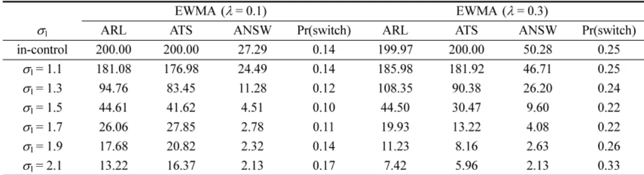
Table 1. Performances of EWMA chart based on Wi when in 0 is changed.
EWMA ( = 0.1) EWM A ( = 0.3)
1 ARL ATS ANSW Pr(switch) ARL ATS ANSW Pr(switch)
in-control 200.00 200.00 27.29 0.14 199.97 200.00 50.28 0.25 1= 1.1 181.08 176.98 24.49 0.14 185.98 181.92 46.71 0.25 1= 1.3 94.76 83.45 11.28 0.12 108.35 90.38 26.20 0.24 1= 1.5 44.61 41.62 4.51 0.10 44.50 30.47 9.60 0.22 1= 1.7 26.06 27.85 2.78 0.11 19.93 13.22 4.08 0.22 1= 1.9 17.68 20.82 2.32 0.14 11.23 8.16 2.63 0.26 1= 2.1 13.22 16.37 2.13 0.17 7.42 5.96 2.13 0.33
Table 2. Performances of CUSUM chart based on Wi when in 0 is changed.
CUSUM (kW= 16.0) CUSUM (kW= 17.0)
1 ARL ATS ANSW Pr(switch) ARL ATS ANSW Pr(switch)
in-control 200.00 199.99 25.93 0.13 200.00 200.02 42.16 0.21 1= 1.1 177.28 171.53 22.91 0.13 180.25 175.76 37.85 0.21 1= 1.3 80.01 61.79 10.03 0.13 85.72 69.09 17.10 0.20 1= 1.5 33.25 20.46 4.27 0.13 32.81 19.90 6.00 0.19 1= 1.7 17.46 9.90 2.69 0.16 15.51 8.04 2.99 0.21 1= 1.9 11.00 6.11 2.14 0.21 9.20 4.59 2.07 0.25 1= 2.1 7.69 4.25 1.82 0.27 6.30 3.17 1.65 0.31 12 12
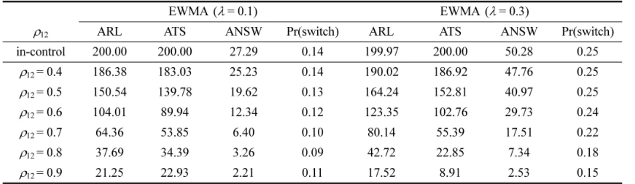
Table 3. Performances of EWMA chart based on Wi when 12 in 0 is changed.
EWMA ( = 0.1) EWM A ( = 0.3)
12 ARL ATS ANSW Pr(switch) ARL ATS ANSW Pr(switch)
in-control 200.00 200.00 27.29 0.14 199.97 200.00 50.28 0.25 12= 0.4 186.38 183.03 25.23 0.14 190.02 186.92 47.76 0.25 12= 0.5 150.54 139.78 19.62 0.13 164.24 152.81 40.97 0.25 12= 0.6 104.01 89.94 12.34 0.12 123.35 102.76 29.73 0.24 12= 0.7 64.36 53.85 6.40 0.10 80.14 55.39 17.51 0.22 12= 0.8 37.69 34.39 3.26 0.09 42.72 22.85 7.34 0.18 12= 0.9 21.25 22.93 2.21 0.11 17.52 8.91 2.53 0.15
Table 4. Performances of CUSUM chart based on Wi when 12 in 0 is changed.
CUSUM (kW= 16.0) CUSUM (kW= 17.0)
12 ARL ATS ANSW Pr(switch) ARL ATS ANSW Pr(switch)
in-control 200.00 199.99 25.93 0.13 200.00 200.02 42.16 0.21 12= 0.4 182.96 178.49 23.68 0.13 186.78 183.35 39.22 0.21 12= 0.5 138.39 124.84 17.62 0.13 148.12 136.71 30.58 0.21 12= 0.6 88.07 68.78 10.87 0.13 98.07 80.07 19.38 0.20 12= 0.7 49.08 31.80 5.79 0.12 53.87 35.75 9.74 0.18 12= 0.8 26.37 14.65 3.26 0.13 26.21 13.25 4.23 0.17 12= 0.9 13.33 6.72 2.13 0.17 11.63 4.70 2.01 0.19
Table 5. Performances of EWMA chart based on Wi when (1, 12) in 0 are changed.
EWMA ( = 0.1) EWM A ( = 0.3)
(1, 12) ARL ATS ANSW Pr(switch) ARL ATS ANSW Pr(switch)
in-control 200.00 200.00 27.29 0.14 199.97 200.00 50.28 0.25 (1.1, 0.4) 172.63 166.62 23.17 0.13 179.69 173.71 45.09 0.25 (1.3, 0.5) 83.37 72.91 9.59 0.12 97.01 77.69 23.09 0.24 (1.5, 0.6) 38.29 36.67 3.78 0.10 36.86 23.96 7.59 0.21 (1.7, 0.7) 22.02 24.45 2.50 0.12 15.76 10.36 3.21 0.22 (1.9, 0.8) 14.52 17.63 2.14 0.16 8.56 6.38 2.20 0.29 (2.1, 0.9) 9.97 12.65 2.00 0.22 5.26 4.34 1.85 0.43
Table 6. Performances of CUSUM chart based on Wi when (1, 12) in 0 are changed.
CUSUM (kW= 16.0) CUSUM (kW= 17.0)
(1, 12) ARL ATS ANSW Pr(switch) ARL ATS ANSW Pr(switch)
in-control 200.00 199.99 25.93 0.13 200.00 200.02 42.16 0.21 (1.1, 0.4) 166.43 158.27 21.45 0.13 171.29 164.87 35.80 0.21 (1.3, 0.5) 68.36 50.22 8.46 0.13 74.02 56.85 14.45 0.20 (1.5, 0.6) 27.58 16.31 3.64 0.14 26.58 15.11 4.79 0.19 (1.7, 0.7) 14.21 7.86 2.37 0.18 12.31 6.04 2.42 0.21 (1.9, 0.8) 8.58 4.60 1.87 0.25 7.07 3.35 1.71 0.28 (2.1, 0.9) 5.47 2.85 1.53 0.34 4.41 2.06 1.30 0.38
VSI charts are given in Table 1 through Table 8. For the CUSUM chart, our computational results show that large reference value k is efficient for large shifts and smaller reference value k is efficient for small shifts of the process parameters in terms of ARL, ATS and ANSW. In EWMA chart, we also found that smaller values of smoothing constant are more efficient for small changes. Ryu and Wan[11] studied the optimal
selection of reference value k in multivariate CUSUM chart for a mean shift of unknown size.
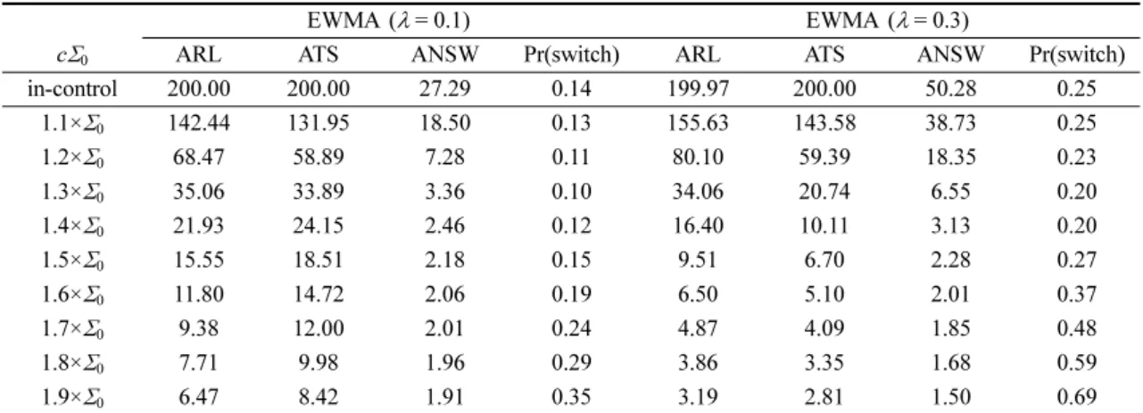
From the simulation results of Table 1 through Table 8, we can see that as the scales of shifts increase the ARL, ATS, and ANSW greatly decrease but the P(swith) dose change a little.
The optimal selection of reference value k in CUSUM or smoothing constant in EWMA charts depend on the size of the shift in monitoring parameters, and so we need to try to find the optimal k and which
fit the scales of shifts of interest.
References
[1] H. Hotelling, “Multivariate quality control”, Tech-niques of Statistical Analysis, McGraw -Hill, New York, pp. 111-184, 1947.
[2] F. B. Alt, “Multivariate quality control” in The Encyclopedia of Statistical Sciences, eds. S. Kotz and Johnson, New York : John Wiley, 1984. [3] J. E. Jackson, “Multivariate quality control”,
Com-munications in Statistics-Theory and Methods, Vol. 14, pp. 2657-2688, 1985.
[4] J. S. Jackson, “Quality control methods for several related variables”, Technometrics, Vol. 1, pp. 359-377, 1959.
[5] P. H. Ghare and P. E. Torgersen, “The multicharac-teristic control chart”, Journal of Industrial Engi-neering, Vol. 19, pp. 269-272, 1968.
Table 7. Performances of EWMA chart based on Wi when 0 is changed to c0.
EWMA ( = 0.1) EWM A ( = 0.3)
c0 ARL ATS ANSW Pr(switch) ARL ATS ANSW Pr(switch)
in-control 200.00 200.00 27.29 0.14 199.97 200.00 50.28 0.25 1.1×0 142.44 131.95 18.50 0.13 155.63 143.58 38.73 0.25 1.2×0 68.47 58.89 7.28 0.11 80.10 59.39 18.35 0.23 1.3×0 35.06 33.89 3.36 0.10 34.06 20.74 6.55 0.20 1.4×0 21.93 24.15 2.46 0.12 16.40 10.11 3.13 0.20 1.5×0 15.55 18.51 2.18 0.15 9.51 6.70 2.28 0.27 1.6×0 11.80 14.72 2.06 0.19 6.50 5.10 2.01 0.37 1.7×0 9.38 12.00 2.01 0.24 4.87 4.09 1.85 0.48 1.8×0 7.71 9.98 1.96 0.29 3.86 3.35 1.68 0.59 1.9×0 6.47 8.42 1.91 0.35 3.19 2.81 1.50 0.69
Table 8. Performances of CUSUM chart based on Wi when 0 is changed to c0.
CUSUM (k = 16.0) CUSUM (k = 17.0)
c0 ARL ATS ANSW Pr(switch) ARL ATS ANSW Pr(switch)
in-control 200.00 199.99 25.93 0.13 200.00 200.02 42.16 0.21 1.1×0 130.15 115.75 16.63 0.13 139.01 126.85 28.67 0.21 1.2×0 53.58 36.16 6.50 0.12 57.71 40.28 10.83 0.19 1.3×0 24.68 14.10 3.28 0.14 23.54 12.47 4.10 0.18 1.4×0 14.09 7.54 2.32 0.18 12.20 5.67 2.33 0.21 1.5×0 9.26 4.80 1.91 0.23 7.67 3.47 1.74 0.26 1.6×0 6.68 3.39 1.66 0.29 5.42 2.46 1.45 0.33 1.7×0 5.10 2.61 1.49 0.36 4.07 1.92 1.26 0.41 1.8×0 4.07 2.07 1.34 0.44 3.24 1.57 1.11 0.50 1.9×0 3.35 1.74 1.21 0.52 2.68 1.38 0.99 0.59
[6] S. W. Roberts, “Control chart tests based on geo-metric moving averages”, Technogeo-metrics, Vol. 1, pp 239-250, 1959.
[7] S. V. Crowder and M. D. Hamilton, “An EWMA for monitoring a process standard deviation”, Jour-nal of Quality Technology, Vol. 24, pp 12-21, 1992. [8] W. H. Woodall and M. M. Ncube, “Multivariate CUSUM quality control procedure”, Technomet-rics, Vol. 27, pp 285-292, 1985.
[9] V. C. C. Vargas, L. F. D. Lopes, and A. M. Sauza, “Comparative study of the performances of the
CuSum and EWMA control charts”, Computer & Industrial Engineering, Vol. 46, pp. 707-724, 2004. [10] D. J. Chang, “Comparison of two sampling intervals and three sampling intervals VSI charts for moni-toring both means and variances”, Journal of the Korean Data & Information Science Society, Vol. 26, pp 997-1006, 2015.
[11] J. H. Ryu and H. Wan, “Optimal design of a CUSUM chart for a mean shift of unknown size”, Journal of Quality Technology, Vol. 42(3), pp. 311-326, 2010.