Multivariate control charts based on regression-adjusted variables for covariance matrix

Multivariate control charts based on regression-adjusted variables for covariance matrix

Bumjun Kwon ¹ · Gyo-Young Cho ²

12 Department of Statistics, Kyungpook National University

Received 29 June 2017, revised 11 July 2017, accepted 15 July 2017

Abstract

The purpose of using a control chart is to detect any change that occurs in the process. When control charts are used to monitor processes, we want to identify this changes as quickly as possible. Many problems in quality control involve a vector of observations of several characteristics rather than a single characteristic. Multivariate CUSUM or EWMA charts have been developed to address the problem of monitoring covariance matrix or the joint monitoring of mean vector and covariance matrix. How- ever, control charts tend to work poorly when we use the highly correlatted variables.

In order to overcome it, Hawkins (1991) proposed the use of regression adjustment vari- ables. In this paper, to monitor covariance matrix, we investigate the performance of MEWMA-type control charts with and without the use of regression adjusted variables.

Keywords: Average run length, covariance matrix, multivariate control chart, regression adjusted variables.

1. Introduction

Many problems in quality control involve a vector of observations of several characteristics rather than a single characteristic. Although one of variables could monitor the process using separate control charts to the extent that these measurements are mutually correlated, it will obtain better sensitivity using multivariate methods that exploit the correlations.

The first multivariate control charts were Shewhart-type charts proposed by Hotelling (1947). CUSUM and EWMA charts are much more effective than Shewhart-type charts for detecting small and moderate shifts in process parameter, and multivariate versions of CUSUM and EWMA charts has been developed. The development of multivariate CUSUM and EWMA charts has concentrated on the problem of monitoring mean vector µ. Jeong and Cho (2012a) studied multivariate Shewhart control charts for the mean vector or covariance matrix. Jeong and Cho (2012b) studied multivariate EWMA control charts for monitoring the covariance matrix. Choi and Cho (2016) studied multivariate CUSUM control charts for monitoring the covariance matrix. Only a few multivariate CUSUM or EWMA charts have

1

Graduate student, Department of Statistics, Kyungpook National University, Daegu 41566, Korea.

2

Corresponding author: Professor, Department of Statistics, Kyungpook National University, Daegu

41566, Korea. E-mail: [email protected]

been developed for the problem of monitoring covariance matrix Σ or the joint monitoring of µ and Σ. But the control charts did not work when we made control charts using the variables that have high correlation. So Hawkins (1991) proposed the use of regression adjustment variables.

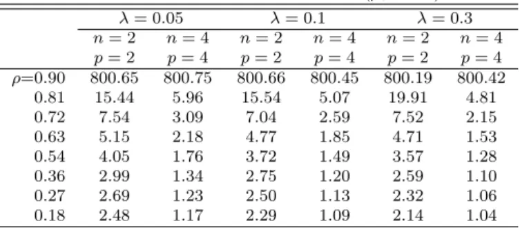
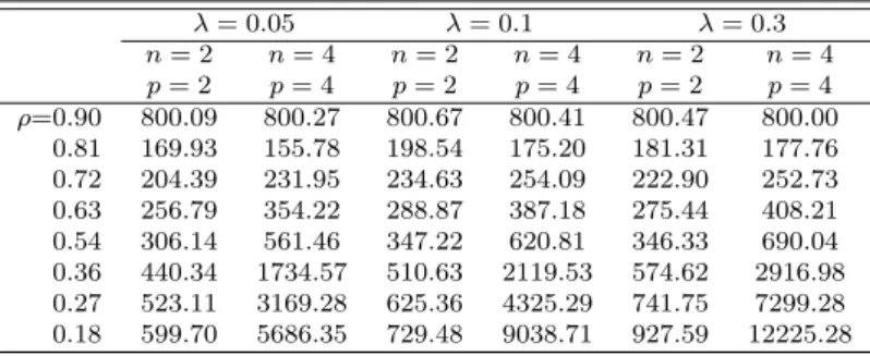
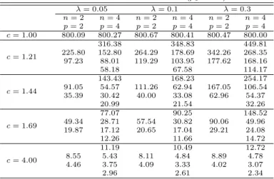
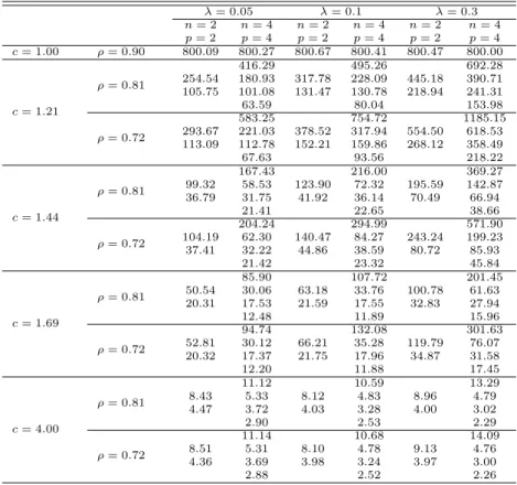
The objective of this paper is to monitor Σ. We use MEWMA-type control charts that are based on the squared deviations of the observations from the target. These control charts were proposed by Reynolds and Cho (2006, 2011). And we have found that the use of regression adjusted variables (Hawkins, 1991, 1993) improves control chart performance in many cases, so we investigate the performance of control charts with and without the use of regression adjusted variables.

2. Definition of control charts

2.1. Notation and assumptions

We suppose that measurement is X, a p-component vector, which is assumed to follow a multivariate normal distribution. It will be convenient to let σ represent the vector of standard deviations of the p variables. Suppose that the objective are to monitor Σ where the target values Σ ₀ , σ ₀ and µ ₀ are known. It is assumed that the in-control process covariance matrix is as follows;

Σ 0 =











1 ρ · · · ρ ρ 1 · · · ρ .. . .. . . . . .. . ρ ρ · · · 1









 .

Assume that the process will be monitored by taking a sample of n ≥ p independent observation vectors at sampling point, where the sampling points are d time units apart.

Let X kij represent observation j (j=1,2,. . .,n) for variable i (i=1,2,. . .,p) at sampling point k (k=1,2,. . .), and let the corresponding standardized observation be

Z _kij = (X kij − µ 0i ) σ _0i ,

where µ 0i is the ith component of µ 0 , and σ 0i is the ith component of σ 0 . Also let z _kj = (Z _k1j Z _k2j · · · Z kpj ), j = 1, 2, . . . , n

be the vector of standardized observations for observations vector j at sampling point k.

Let Σ _Z be the covariance matrix of z _kj , and let Σ _Z0 be the in-control value of Σ _Z . The in-control distribution of Z _kij is standard normal, so Σ _Z0 is also the in-control correlation matrix of the unstandardized observations.

Some control statistics used for monitoring Σ are functions of the sample estimates of Σ Z . At sampling point k, let ˆ Σ Zk be the maximum likelihood estimator of Σ Z , where the (i, i

) element of ˆ Σ _Zk is P n

j=1 Z

Z

ki0j

n .

2.2. Regression adjustment variables

When the variables are highly correlated, however, the performance of control charts will be poorer than that of the best procedures that capitalize on the correlation between variables. The MEWMA can be designed to have faster detection capability. Furthermore Hotelling T ² is not optimal for more structured shifts in the mean, such as shifts in only a few of the process variables. It also turns out that the Hotelling T ² , and any method that uses the quadratic form structure of the Hotelling T ² test statistic (such as MEWMA), will be sensitive to shifts in the variance as well as to shifts in the mean.

Hawkins (1991,1993) has developed a procedure called regression adjustment that is po- tentially very useful. It consists of control charts of the resuduals from each variable obtained when that variable is regressed on all the others. The vector of regression adjusted variables, say a kj = (A k1j A k2j · · · A kpj )

corresponding to the vector of standardized observa- tions z kj , is given by

a kj = (diagΣ ⁻¹ _Z0 ) ⁻

Σ ⁻¹ _Z0 z kj ,

where B = (diagΣ ⁻¹ _Z0 ) ⁻

Σ ⁻¹ _Z0 is said to be transformation matrix and

(diagΣ ⁻¹ _Z0 ) ⁻

=











p 1 − ρ ² 0 · · · 0

0 p

1 − ρ ² · · · 0 .. . .. . . . . .. .

0 0 · · · p

1 − ρ ²









 .

Then a kj has mean µ A = (diagΣ ⁻¹ _Z0 ) ⁻

Σ ⁻¹ _Z0 µ Z , where µ Z = E(z kj ), and covariance matrix Σ A = (diagΣ ⁻¹ _Z0 ) ⁻

Σ ⁻¹ _Z0 Σ Z Σ ⁻¹ _Z0 (diagΣ ⁻¹ _Z0 ) ⁻

. In the in-control case, µ A0 = 0 and Σ A = (diagΣ ⁻¹ _Z0 ) ⁻

Σ ⁻¹ _Z0 (diagΣ ⁻¹ _Z0 ) ⁻

is the correlation matrix of a _kj .

Regression adjustment has some feature. If the proper set of variables is included in the

regression model, the residuals from the model will typically be uncorrelated, even though

the original variable of exhibited correlation variables. And it occurs when the process has

a distinct hierarchy of variables, such as a set of input process variables and a set of out-

put variables. Because of this nice feature, the regression adjustment procedure has many

possible applications in process plants where many of the variables are highly correlated.

2.3. Set of MEWMA control charts

The MEWMA control chart for monitoring Σ is based on EWMA statistic. And we use MEWMA-type statistic based on squared standardized deviations from target which was propesed by Reynolds and Cho (2006). We define two MEWMA-type statistics with and without regression adjustment variables. First, at sampling point k let the EWMA statis- tic of squared standardized deviations from target for normal variable (without regression adjustment) i be

E _ki ^Z = (1 − λ)E _k−1 ^Z + λ(

n

X

j=1

Z _kij ²

n ), i = 1, 2, · · · , p, (2.1) where E _0i ^Z = 1 and 0 < λ ≤ 1.

The first form of MEWMA-type statistic based on E _ki ^Z is M _k ^Z = n

2c k

(E _k1 ^Z − 1, · · · , E _kp ^Z − 1)(Σ ⁽²⁾ _Z0 ) ⁻¹ (E _k1 ^Z − 1, · · · , E _kp ^Z − 1)

, (2.2)

where c k = ^{λ[1−(1−λ)} _(2−λ)

^] , k = 1, 2, · · · . This statistic is used with a UCL and will be called the MZ chart. The MZ statistic follows the standard form of an MEWMA in the sense that the in-control mean is subtracted from each E _ki ^Z .

Second, The MEWMA charts based on the squared deviations of the regression adjusted variables from target are defined with the components of a kj used in place of the components of z kj , and Σ Z0 replaced with Σ A0 . At sampling point k let the EWMA statistic of squared standardized deviations from target for regression adjustment variable i be

E _ki ^A = (1 − λ)E _k−1 ^A + λ(

n

X

j=1

A ² _kij

n ), i = 1, 2, · · · , p, (2.3) where E _0i ^A = 1 and 0 < λ ≤ 1.

The form of MEWMA-type statistic based on E _ki ^A is M _k ^A = 2c _k

n (E _k1 ^A − 1, · · · , E _kp ^A − 1)(Σ ⁽²⁾ _A0 ) ⁻¹ (E _k1 ^A − 1, · · · , E _kp ^A − 1)

, (2.4) where c k = ^{λ[1−(1−λ)} _(2−λ)

^] , k = 1, 2, · · · .

This statistic is also used with a UCL and will be called the MA chart. The MA statistic follows the standard form of an MEWMA in the sense that the in-control mean is subtracted from each E _ki ^A . The control charts based on squared deviations from target are very effective for detecting chages in Σ.

2.4. Measures of control chart performance

We will compare multivariate control charts in terms of the ARL (Average run length)

required to detect shifts in process parameters, when each chart has the same false alarm

rate. If there is a shift in a process parameter, the ARL is the appropriate measure of

detection time for this shift.

The Markov chain and integral equation methods can be used to evaluate properties of the multivariate EWMA chart (Rigdon (1995a, b), Prabhu and Runger (1997)), but it is not feasible to use these methods for the regression adjustment of charts. Thus simulation with 5,000 runs was used. All of the schemes being compared have an in-control ARL of 800 hours where the sampling interval d is assumed to be 1 hour.

3. Numerical results

When the production process changes, the following types of shifts in the covariance matrix Σ are considered; (1) covariances are changed and variances are not changed, (2) variances are changed and covariances are not changed, (3) variances and covariances are simultaneously changed.

The ability of a control chart to detect any shifts in the production process is determined by the length of time required to signal. Thus, a good control chart detects shifts quickly in the process when the process is out-of-control state, and produce few false alarms when the process is in-control state.

Table 3.1 Values of h when the in-control ARL is approximately 800

λ=0.05 λ=0.1 λ=0.3

MA chart n = 2, p = 2 28.7697 39.7537 69.7074 n = 4, p = 4 22.1106 27.1261 40.5803 MZ chart n = 2, p = 2 28.9519 39.8798 69.6477 n = 4, p = 4 98.7886 127.2629 204.0411

The control limits h and ARLs for multivariate EWMA control charts are obtained by using 5,000 runs. Table 3.1 gives the values of h for p = 2, 4 λ = 0.05, 0.1, 0.3 when the in-control ARL is approximately 800.

3.1. Changes in covariances

Table 3.2 MA charts for covariances (ρ

= 0.9)

λ = 0.05 λ = 0.1 λ = 0.3

n = 2 n = 4 n = 2 n = 4 n = 2 n = 4 p = 2 p = 4 p = 2 p = 4 p = 2 p = 4 ρ=0.90 800.65 800.75 800.66 800.45 800.19 800.42

0.81 15.44 5.96 15.54 5.07 19.91 4.81

0.72 7.54 3.09 7.04 2.59 7.52 2.15

0.63 5.15 2.18 4.77 1.85 4.71 1.53

0.54 4.05 1.76 3.72 1.49 3.57 1.28

0.36 2.99 1.34 2.75 1.20 2.59 1.10

0.27 2.69 1.23 2.50 1.13 2.32 1.06

0.18 2.48 1.17 2.29 1.09 2.14 1.04

Tables 3.2 and 3.3 give the ARLs of MA charts and MZ charts for n = 2, 4 and p = 2, 4 when covariances are changed and variances are not changed. Here the changed values of ρ considered in Tables 3.2 and 3.3 are those of decreased from 0.9 to 0.18, respectively.

As shown in Table 3.2 the MA charts for monitoring the covariance matrix are effective in

Table 3.3 MZ charts for covariances (ρ

= 0.9)

λ = 0.05 λ = 0.1 λ = 0.3

n = 2 n = 4 n = 2 n = 4 n = 2 n = 4

p = 2 p = 4 p = 2 p = 4 p = 2 p = 4

ρ=0.90 800.09 800.27 800.67 800.41 800.47 800.00 0.81 169.93 155.78 198.54 175.20 181.31 177.76 0.72 204.39 231.95 234.63 254.09 222.90 252.73 0.63 256.79 354.22 288.87 387.18 275.44 408.21 0.54 306.14 561.46 347.22 620.81 346.33 690.04 0.36 440.34 1734.57 510.63 2119.53 574.62 2916.98 0.27 523.11 3169.28 625.36 4325.29 741.75 7299.28 0.18 599.70 5686.35 729.48 9038.71 927.59 12225.28

detecting only changes in covariance. On the other hand, shown in Table 3.3 the ARLs of MZ charts for monitoring the covariance matrix is increased by changing ρ.

3.2. Changes in variances

Table 3.4 MA charts for variances (ρ

= 0.9)

λ = 0.05 λ = 0.1 λ = 0.3

n = 2 n = 4 n = 2 n = 4 n = 2 n = 4 p = 2 p = 4 p = 2 p = 4 p = 2 p = 4 c = 1.00 800.65 800.75 800.66 800.45 800.19 800.42 c = 1.21

149.47 179.38 270.00

154.59 64.12 182.33 76.73 259.90 136.66 97.27 42.01 119.85 48.51 181.05 90.08

33.91 37.44 68.37

c = 1.44

35.36 38.21 60.88

41.05 17.60 46.63 17.13 73.28 24.69 35.16 13.62 39.67 12.72 62.71 17.37

12.91 12.02 15.87

c = 1.69

15.41 14.35 18.15

18.49 8.84 18.88 7.72 25.50 8.27

19.75 7.46 20.45 6.48 28.93 6.63

7.82 6.78 7.09

c = 4.00

2.09 1.82 1.58

2.75 1.57 2.55 1.39 2.38 1.24

4.48 1.52 4.09 1.33 4.02 1.18

1.99 1.69 1.42

Tables 3.4 and 3.5 give p ARLs of MA charts and MZ charts for n = 2, 4 and p = 2, 4 when variances are changed and covariances are not changed. In each cell, there are p ARLs when 1, 2, · · · , p variances are changed, respectively. Here standard deviations are changed from σ ₀ to σ = √

cσ ₀ for c = 1.21, 1.44, 1.69, 4.00. As shown in Tables 3.4

and 3.5, MA charts are effective in detecting changes in variances.

Table 3.5 MZ charts for variances (ρ

= 0.9)

λ = 0.05 λ = 0.1 λ = 0.3

n = 2 n = 4 n = 2 n = 4 n = 2 n = 4 p = 2 p = 4 p = 2 p = 4 p = 2 p = 4 c = 1.00 800.09 800.27 800.67 800.41 800.47 800.00 c = 1.21

316.38 348.83 449.81

225.80 152.80 264.29 178.69 342.26 268.35 97.23 88.01 119.29 103.95 177.62 168.16

58.18 67.58 114.17

c = 1.44

143.43 168.23 254.17

91.05 54.57 111.26 62.94 167.05 106.54 35.39 30.42 40.00 33.08 62.96 54.37

20.99 21.54 32.26

c = 1.69

77.07 90.25 148.52

49.34 28.71 57.54 30.82 90.06 49.96 19.87 17.12 20.65 17.04 29.21 24.08

12.26 11.66 14.72

c = 4.00

11.19 10.49 12.72

8.55 5.43 8.11 4.84 8.89 4.78

4.46 3.75 4.09 3.33 4.02 3.07

2.96 2.61 2.34

3.3. Changse in variances and covariances

Table 3.6 MA charts for variances and covariances (ρ

= 0.9)

λ = 0.05 λ = 0.1 λ = 0.3

n = 2 n = 4 n = 2 n = 4 n = 2 n = 4 p = 2 p = 4 p = 2 p = 4 p = 2 p = 4 c = 1.00 ρ = 0.90 800.65 800.75 800.66 800.45 800.19 800.42

c = 1.21

ρ = 0.81

5.30 4.43 4.00

11.94 4.78 11.47 3.99 13.99 3.51

10.25 4.43 10.00 3.72 11.69 3.22

4.14 3.47 3.02

ρ = 0.72

2.86 2.38 1.98

6.35 2.69 5.92 2.24 6.12 1.85

5.69 2.54 5.27 2.12 5.37 1.76

2.41 2.03 1.67

c = 1.44

ρ = 0.81

4.56 3.80 3.35

9.06 3.80 8.44 3.20 9.64 2.72

7.65 3.41 7.17 2.85 7.72 2.40

3.15 2.64 2.22

ρ = 0.72

2.63 2.18 1.82

5.38 2.30 4.95 1.95 4.94 1.62

4.65 2.12 4.27 1.80 4.17 1.49

1.99 1.69 1.41

c = 1.69

ρ = 0.81

3.86 3.22 2.74

6.97 3.08 6.51 2.58 6.90 2.14

5.99 2.71 5.63 2.26 5.72 1.91

2.56 2.15 1.78

ρ = 0.72

2.37 1.99 1.67

4.58 2.02 4.19 1.72 4.09 1.44

3.89 1.83 3.57 1.55 3.43 1.32

1.71 1.46 1.26

c = 4.00

ρ = 0.81

1.61 1.45 1.27

2.37 1.27 2.17 1.16 2.03 1.08

2.57 1.17 2.34 1.09 2.19 1.03

1.21 1.10 1.05

ρ = 0.72

1.39 1.26 1.14

2.08 1.13 1.93 1.07 1.81 1.03

1.99 1.06 1.86 1.03 1.75 1.01

1.05 1.02 1.00

Table 3.7 MZ charts for variances and covariances (ρ

= 0.9)

λ = 0.05 λ = 0.1 λ = 0.3

n = 2 n = 4 n = 2 n = 4 n = 2 n = 4 p = 2 p = 4 p = 2 p = 4 p = 2 p = 4 c = 1.00 ρ = 0.90 800.09 800.27 800.67 800.41 800.47 800.00

c = 1.21

ρ = 0.81

416.29 495.26 692.28

254.54 180.93 317.78 228.09 445.18 390.71 105.75 101.08 131.47 130.78 218.94 241.31

63.59 80.04 153.98

ρ = 0.72

583.25 754.72 1185.15

293.67 221.03 378.52 317.94 554.50 618.53 113.09 112.78 152.21 159.86 268.12 358.49

67.63 93.56 218.22

c = 1.44

ρ = 0.81

167.43 216.00 369.27

99.32 58.53 123.90 72.32 195.59 142.87 36.79 31.75 41.92 36.14 70.49 66.94

21.41 22.65 38.66

ρ = 0.72

204.24 294.99 571.90

104.19 62.30 140.47 84.27 243.24 199.23 37.41 32.22 44.86 38.59 80.72 85.93

21.42 23.32 45.84

c = 1.69

ρ = 0.81

85.90 107.72 201.45

50.54 30.06 63.18 33.76 100.78 61.63 20.31 17.53 21.59 17.55 32.83 27.94

12.48 11.89 15.96

ρ = 0.72

94.74 132.08 301.63

52.81 30.12 66.21 35.28 119.79 76.07 20.32 17.37 21.75 17.96 34.87 31.58

12.20 11.88 17.45

c = 4.00

ρ = 0.81

11.12 10.59 13.29

8.43 5.33 8.12 4.83 8.96 4.79

4.47 3.72 4.03 3.28 4.00 3.02

2.90 2.53 2.29

ρ = 0.72

11.14 10.68 14.09

8.51 5.31 8.10 4.78 9.13 4.76

4.36 3.69 3.98 3.24 3.97 3.00

2.88 2.52 2.26

For n = 2, 4 and p = 2, 4, Tables 3.6 and 3.7 give p ARLs in each cell when 1, 2, · · · , p variances and p covariances are simultaneously changed, respectively. Here standard devia- tions are changed from σ 0 to σ = √

cσ 0 for c = 1.21, 1.44, 1.69, 4.00 and covariances are changed from ρ ₀ = 0.9 to ρ = 0.81, 0.72. As shown in Tables 3.6 and 3.7, MA charts are effective in detecting changes in variances and covariances.

4. Summary and concluding remark

This paper is a study on the multivariate EWMA control charts for monitoring covariance matrix. These multivariate control charts are constructed by using the two different control statistics which are based on squared deviations with and without regression adjustment variables from target variables.

We consider MEWMA-type control charts for n = 2, 4, p = 2, 4, ρ ₀ = 0.9 and λ = 0.05, 0.10, 0.30. We can get control limits and ARLs of the proposed multivariate control charts by using simulations. The performance of these proposed multivariate control charts is compared with their ARLs.

The objective of monitoring is assumed to be the detection of small as well as large shifts

in changes Σ and as quickly as highly correlated variables shifts. The conclusions from this

investigation can be summarized as follows. As shown Tables 3.2-3.7, we can confirm that MA charts based on squared deviations using regression adjustment variables from target will effectively detect in Σ than MZ charts. Also using regression adjustment of the variables improves overall performance when the variables are correlated. The MA chart based on regression adjustment variables from target are recommended here because they offer very fast detection of changes in Σ and good working when exist highly correlated variables.

References

Choi, H. Y. and Cho, G. Y. (2016). Multivariate CUSUM control charts for monitoring the covariance matrix. Journal of the Korean Data & Information Science Society, 27, 539-548.

Hawkins, D. M. (1991). Multivariate quality control based on regression-adjusted variables. Technometrics, 33, 61-75

Hawkins, D. M. (1993). Regression adjustment for variables in multivariate quality control. Journal of Quality Technology, 25, 170-182.

Hotelling, H. (1947). Multivariate quality control-illustrated by the air testing of sample bombsights in techniques of statistical analysis edited by C. Eisenhart, M.W. Hastay, and W.A. Wallis, McGraw- Hill, New York.

Jeong, J. I. and Cho, G. Y. (2012a). Multivariate Shewhart control charts for monitoring the vatiance- covariance matrix. Journal of the Korean Data & Information Science Society, 23, 617-626.

Jeong, J. I. and Cho, G. Y. (2012b). Multivariate EWMA control charts for monitoring the variance- covariance matrix. Journal of the Korean Data & Information Science Society, 23, 807-814.

Lowry, C. A., Woodall, W. H., Champ, C. W. and Rigdon, S. E. (1992). A multivariate exponentially weighted moving average control chart. Technometrics, 34, 46-53.

Prabhu, S. S. and Runger, G. C. (1997). Designing a multivariate EWMA control chart. Journal of Quality Technology, 29, 8-15.

Rigdon, S. E. (1995a). An integral equation for the in-control average run length of a multivariate expo- nentially weighted moving average control chart. Journal of Statistical Computation and Simulation, 52, 351-365.

Rigdon, S. E. (1995b). A double-integral equation for the average run length of a multivariate exponentially weighted moving average control chart. Statistics and Probability Letters, 24, 365-373.

Reynolds, M. R., Jr. and Cho, G. Y. (2006). Multivariate control charts for monitoring the mean vector and covariance matrix. Sequential Analysis, 30, 1-40.

Reynolds, M. R., Jr. and Cho, G. Y. (2011). Multivariate control charts for monitoring the mean vector

and covariance matrix with variable sampling intervals. Sequential Analysis, 30, 1-40.