Switching properties of bivariate Shewhart control charts for monitoring the covariance matrix
Hyeon Jin Gwon 1 · Gyo-Young Cho 2
12 Department of Statistics, Kyungpook National University
Received 29 October 2015, revised 18 November 2015, accepted 24 November 2015
Abstract
A control chart is very useful in monitoring various production process. There are many situations in which the simultaneous control of two or more related quality vari- ables is necessary. We construct bivariate Shewhart control charts based on the trace of the product of the estimated variance-covariance matrix and the inverse of the in-control matrix and investigate the properties of bivariate Shewart control charts with VSI pro- cedure for monitoring covariance matrix in term of ATS (Average time to signal) and ANSW (Average number of switch) and probability of switch, ASI (Average sampling interval). Numerical results show that ATS is smaller than ARL. From examining the properties of switching in changing covariances and variances in Σ, ANSW values show that it does not switch frequently and does not matter to use VSI procedure.
Keywords: Average run length, average number of switches, average sampling interval, average time to signal, switching property.
1. Introduction
The purpose of a control chart is to detect assignable causes of variation that occur in the process. During the control process, we want to detect any departure from in-control state and find this change as quickly as possible. For a good control chart, it can be aware of a shift quickly in the process when the process is out-of-control state and generate few false alarms when the process is in-control state.
There are many problems in the quality control that imply a vector of measurements of several quality variables rather than a single quality variable. If the quality variables are correlated, it has better sensitivity by using multivariate control charts.
For control charts, it takes samples from the process at fixed sampling interval (FSI).
FSI procedures are simple and very popular, but we can change time interval as a function of what is observed from the process. Strategy of changing time interval is called variable sampling interval (VSI). Under the VSI procedures, when there is an indication of the process change, the time interval would be short.
VSI procedures were first investigated by Arnold (1970) and his works were extended by Smeach and Jernigan (1977). Also Reynolds and Arnold (1989) developed general expressions
1
Graduate student, Department of Statistics, Kyungpook National University, Daegu, 702-701, Korea.
2
Corresponding author: Professor, Department of Statistics, Kyungpook National University, Daegu,
702-701, Korea. E-mail: [email protected]
such as ARL and ATS for VSI control charts. But VSI procedures have a disadvantage that is frequent switching between different sampling intervals which requires more cost and effort to administer the process than corresponding FSI procedures. Amin and Letsinger (1991) studied switching behavior and run rules for switching between different sampling intervals.
Amin and Hemasinha (1993) developed expression for the ANSW and ATS for VSI ¯ X -chart for evaluating the switching behavior.
In this paper, we investigate the properties of bivariate Shewart charts with VSI procedure for monitoring covariance matrix in term of ATS (Average Time to Signal) and ANSW (Average number of Switch) and probability of switch, ASI (Average sampling interval).
In Section 2, we introduce notation, assumptions and properties of VSI procedures. And we construct bivariate Shewhart control charts based on the trace of the product of the estimated variance-covariance matrix and the inverse of the in-control matrix. In Section 3, we simulate bivariate control charts with three types of sifts in the covariance matrix.
2. Description of control procedures
Suppose that the process of interest has p quality variables presented by the random vector X 0 = (X 1 , X 2 , · · · , X p ) and we take a sequence of samples of size n at each sampling occasion i (i = 1, 2, · · · ). It will be assumed that the successive observation vectors are independent and have bivariate normal distribution with N p (µ, Σ) where the mean vector µ = µ 0 is known.
2.1. Evaluating sample statistic
Suppose that the process of interest has p quality variables whose distribution is bivariate normal with mean vector µ and covariance matrix Σ where the mean vector µ = µ 0 is known.
It will be convenient to let σ represent the vector of standard deviations of the variable. Let µ 0 , Σ 0 and σ 0 be the in-control values of µ, Σ and σ. We will usually refer to Σ 0 as target, even though, in practice, some of the components of Σ 0 may correspond to estimated values rather than specified target value.
We take a sequence of random samples of size n ≥ p at each sampling point, where the sampling points are d time units apart. Let X kij be the jth observation for variable i at sampling point k for k = 1, 2, · · · , i = 1, 2, · · · , p and j = 1, 2, · · · , n, and let the corresponding standardized observation be
Z kij = (X kij − µ 0i )/σ 0i
where µ 0i is the ith component of µ 0 and σ 0i is the ith component of σ 0 . Also let Z kj = (Z k1j , Z k2j , · · · , Z kpj )
0, j = 1, 2, · · · , n
be the vector of standardized observations for observation vector j at sampling point k.
Let Σ Z be the covariance matrix of Z kj , and let Σ Z0 be the in-control value of Σ Z . The in-control distribution of Z kij is standard normal, so Σ Z0 is also the in-control correlation matrix of the unstandardized observations. When n ≥ p, some control statistics used for monitoring Σ are functions of the sample estimates b Σ Z . At sampling point k, let b Σ Zk be the maximum likelihood estimator of Σ Z , where the (i, i
0) element of b Σ Zk is P n
j=1 Z kij Z ki
0j /n.
2.2. Properties of VSI procedures
The basic idea of VSI control charts is that if there is some indication of a process change, the time interval would be short and it would be long if not. For VSI charts, the sampling intervals are random variable and the sampling interval depends on the past sample infor- mations of X 1 , X 2 , · · · , X i . Reynolds (1989) investigated the theoretical aspects of a VSI two-sided control charts. Reynolds and Arnold (1989) investigated the theoretical aspects of a VSI one-sided Shewhart control charts. Reynolds (1995) evaluated properties of variable sampling interval control charts. Chang and Heo (2012) investgated switching properties of CUSUM charts for controlling mean vector. Reynolds and Stoumbos (2001) studied on mon- itoring the process mean and variance using individual observations and variable sampling intervals. Chang and Cho (2005) studied CUSUM charts for monitoring mean vector with variable sampling intervals. Reynolds and Cho (2006), Reynolds and Cho (2011), Jeong and Cho (2012) studied multivariate control charts for the mean vector or covariance matrix.
To implement two sampling interval control charts, there are two disjoint regions I 1 , I 2 that divide the in-control region. I i is the region in which the sampling interval d i is used (i = 1, 2).
In this paper, we assume that the VSI chart starts at time 0 and the interval used before the first sample, is a fixed constant, say d 0 . Then the ARL and ATS can be expressed as
( ARL = 1 + ψ 1 + ψ 2 AT S = d 0 + d 1 ψ 1 + d 2 ψ 2
where ψ i is the expected number of samples before the signal. Also ATS can be expressed as AT S = d · ARL and d can be interpreted as the average sampling interval (ASI) of the charts to signal. And ρ 1 can be interpreted as the long-run proportion of sampling interval that d 1 is used where
d = d 1 ρ 1 + d 2 (1 − ρ 1 )
The VSI procedures are substantially more efficient than FSI procedures in the term of ARL and ATS. But, the ARL and ATS do not show any switching information between the different sampling intervals d 1 and d 2 . Therefore, it is necessary to define the number of switches (NSW) as the number of switches made from the start of the process until the chart signals, and let average number of switches (ANSW) be the expected value of the NSW.
The ANSW can be obtained as follows
AN SW = N SW · P (switches) And, the probability of switch is given by
P (switch) = P (d 1 ) · P (d 2 |d 1 ) + P (d 2 ) · P (d 1 |d 2 )
where p(d i ) is the probability of using sampling interval d i , and p(d i |d j ) is the conditional probability of using sampling interval d i in the current sample given that the sampling interval d j (d i 6= d j ) was used in the previous sample.
By Amin and Lestinger (1991), the number of samples taken from the time the process
starts using the sampling interval d i until a switch is made to sampling interval d j (i 6= j),
and let average number of samples until a switch (ANSSW) be the expected value of the
number of samples until a switch.
2.3. Bivariate Shewhart control chart
Reynolds and Stoumbos (2004a, 2004b) suggested that Shewhart control charts are very sensitive to the choice of the sample size. So, Shewhart control chart is one of the most widely used control charts for monitoring the production process. A Shewhart control chart can detect large changes in monitored parameter quickly. But Shewhart control chart is relatively inefficient in detecting small shift in control parameter, because it uses only the information in the current sample. We can obtain a sample statistic for monitoring covariance matrix by using the statistic for testing
H 0 : Σ = Σ 0 vs H 1 : Σ 6= Σ 0 .
The Shewhart-type control chart proposed by Hotelling (1947) for monitoring mean vector µ (frequently called Hotelling’s T 2 chart) was originally developed for the case in which Σ 0 is unknown. If Σ 0 is assumed to be known, then this control chart is equivalent to a control chart based on the statistic used with an upper control limit (UCL).
(Z k1 , Z k2 , · · · Z kp )Σ −1 ZO (Z k1 , Z k2 , · · · Z kp ) 0 Hotelling(1947) proposed a control chart for monitoring Σ based on
n
X
j=1
(Z kij , Z k2j , · · · , Z kpj )Σ −1 Z0 (Z kij , Z k2j , · · · , Z kpj ) 0 = ntr( d Σ Zk Σ −1 Z0 ) = Y k.
This control chart has both a lower control limit (LCL) and an UCL.
For the VSI Shewhart control chart based on Y k , suppose that the sampling interval;
d 1 is used when Y k ∈ (g Y
k, h Y
k], d 2 is used when Y k ∈ (0, g Y
k], where g Y
k≤ h Y
kand d 1 < d 2 .
The percentage point of Y k can be obtained from the chi-square distribution when the process is in-control. If the process is in-control, the statistic Y k has a chi-squared distribution with p degree of freedom. Hence, the design parameters g Y
kand h Y
kcan be obtained to satisfy a desired ARL and ATS.
3. Numerical result and concluding remarks
The ability of a control chart to detect any shifts in the production process is determined by the length of time required to signal. Thus, a good control chart detects shifts as quickly as possible at out-of-control state and produce few alarms at in-control state.
In evaluating the properties of the VSI procedure, we compare the performance of the VSI to the same procedure using FSI procedure. Also, we will use process parameters based on ATS and ARL.
In order to evaluate the performances and compare the proposed bivariate Shewhart con-
trol charts fairly, some kinds of standards for comparison are necessary. In our computa-
tion, each control chart has been set so that on-target ARL and ATS were approximately
equal to 800.0 and the sample size for each control chart was 2, 4 for p = 2. And we used
d 0 = 0, d 1 = 1.9, d 2 = 0.1. The performance of the charts for monitoring the covariance
matrix depends on the value of Σ. The following types of shifts were considered
(1) variances are changed and covariances are not changed, (2) covariances are changed and variances are not changed, (3) variances and covariances are simultaneously changed.
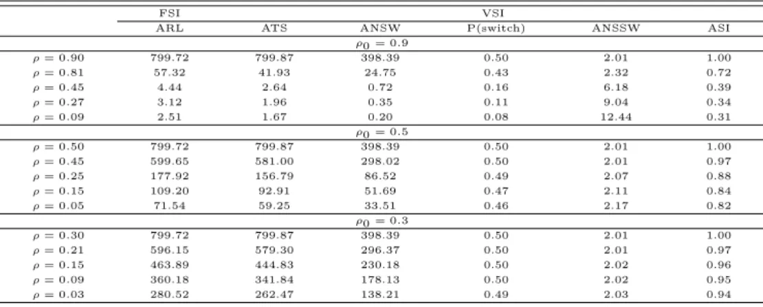
Tables 3.1-3.2 give the values of and ARL and ATS, ANSW, P (switch), ANSSW, ASI for n = 2, 4 and p = 2 and three different in-control correlation coefficients ρ 0 = 0.9, 0.5, 0.3 when covariances are changed and variance are not changed. Here the changed value con- sidered in Tables 3.1-3.2 are those of decreased by 10%, 50%, 70% and 90% of ρ 0 values, respectively. As shown in Tables 3.1-3.2, the bivariate Shewharts control chart proposed by Hotelling (1947) for monitoring the variance-covariance matrix are effective in detecting changes of covariances in Σ.
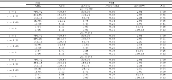
Tables 3.3-3.4 give the values of ARL, ATS, ANSW, P (switch), ANSSW, ASI for n = 2, 4 and p = 2 when variances are changed and covariances are not changed, respectively. Here the variances are changed from σ = √
cσ 0 , for c =1.21, 1.44, 1.69, 4. As shown in Tables 3.3-3.4, the bivariate Shewharts control chart proposed by Hotelling (1947) for monitoring the variance-covariance matrix are effective in detecting changes of variances in Σ.
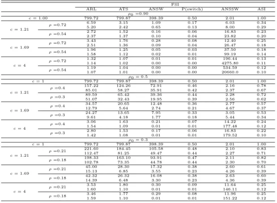
For n = 2, 4 and p = 2, Tables 3.5-3.6 give ARL, ATS, ANSW, P (switch), ANSSW, ASI in each cell when only 2 variances and covariances are simultaneously changed respectively.
Here the variances are changed from σ = √
cσ 0 , for c=1.21, 1.44, 1.69, 4. And covariances are also changed from ρ 0 = 0.9 to ρ 0 = 0.72, 0.54, ρ 0 = 0.5 to ρ 0 = 0.4, 0.3 and ρ 0 = 0.3 to ρ 0 = 0.21, 0.8. As shown in Tables 3.5-3.6, the bivariate Shewharts control chart proposed by Hotelling (1947) for monitoring the variance-covariance matrix are effective in detecting simultaneously changes of variance and covariance in Σ.
Numerical results for various tables give ARL, ATS, ANSW, P (switch), ANSSW, ASI.
First, we realize that ATS is smaller than ARL. That means VSI control chart is faster than FSI control chart for detecting variations in the production process. Second, we examine the properties of switching in changing covariances and variances in Σ. ANSW values show that it does not switch frequently and does not matter to use VSI procedure.
Table 3.1 ARL and ATS, ANSW, P (switch), ANSSW, ASI when covariances are changed and variance are not changed (n=2, p=2)
FSI VSI
ARL ATS ANSW P(switch) ANSSW ASI
ρ0 = 0.9
ρ = 0.90 799.72 799.87 398.39 0.50 2.01 1.00
ρ = 0.81 57.32 41.93 24.75 0.43 2.32 0.72
ρ = 0.45 4.44 2.64 0.72 0.16 6.18 0.39
ρ = 0.27 3.12 1.96 0.35 0.11 9.04 0.34
ρ = 0.09 2.51 1.67 0.20 0.08 12.44 0.31
ρ0 = 0.5
ρ = 0.50 799.72 799.87 398.39 0.50 2.01 1.00
ρ = 0.45 599.65 581.00 298.02 0.50 2.01 0.97
ρ = 0.25 177.92 156.79 86.52 0.49 2.07 0.88
ρ = 0.15 109.20 92.91 51.69 0.47 2.11 0.84
ρ = 0.05 71.54 59.25 33.51 0.46 2.17 0.82
ρ0 = 0.3
ρ = 0.30 799.72 799.87 398.39 0.50 2.01 1.00
ρ = 0.21 596.15 579.30 296.37 0.50 2.01 0.97
ρ = 0.15 463.89 444.83 230.18 0.50 2.02 0.96
ρ = 0.09 360.18 341.84 178.13 0.50 2.02 0.95
ρ = 0.03 280.52 262.47 138.21 0.49 2.03 0.94
Table 3.2 ARL and ATS, ANSW, P (switch), ANSSW, ASI when covariances are changed and variance are not changed (n=4, p=2)
FSI VSI
ARL ATS ANSW P(switch) ANSSW ASI
ρ0 = 0.9
ρ = 0.90 799.72 799.87 398.39 0.50 2.01 1.00
ρ = 0.81 36.11 22.21 13.39 0.37 2.70 0.59
ρ = 0.45 2.54 1.48 0.14 0.06 18.07 0.23
ρ = 0.27 1.86 1.25 0.05 0.03 38.23 0.19
ρ = 0.09 1.57 1.16 0.02 0.01 72.52 0.16
ρ0 = 0.5
ρ = 0.50 799.72 799.87 398.39 0.50 2.01 1.00
ρ = 0.45 551.93 527.57 273.81 0.50 2.02 0.95
ρ = 0.25 141.12 114.59 65.76 0.47 2.13 0.81
ρ = 0.15 80.35 61.81 36.16 0.45 2.22 0.76
ρ = 0.05 50.69 37.11 21.70 0.43 2.34 0.71
ρ0 = 0.3
ρ = 0.30 799.72 799.87 398.39 0.50 2.01 1.00
ρ = 0.21 595.15 580.30 295.88 0.50 2.01 0.50
ρ = 0.15 429.96 404.00 212.48 0.49 2.02 0.94
ρ = 0.09 327.54 301.15 160.99 0.49 2.04 0.92
ρ = 0.03 248.17 223.83 121.17 0.49 2.05 0.90
Table 3.3 ARL and ATS, ANSW, P (switch), ANSSW, ASI when variances are changed and covariances are not changed (n=2, p=2)
FSI
ARL ATS ANSW P(switch) ANSSW ASI
ρ0 = 0.90
c = 1 799.72 799.87 398.39 0.50 2.01 1.00
c = 1.21 253.97 229.31 124.10 0.49 2.05 0.90
198.31 164.53 94.25 0.48 2.10 0.83
c = 1.69 31.48 23.04 12.95 0.41 2.43 0.70
32.47 19.30 11.59 0.36 2.80 0.57
c = 4 2.64 1.77 0.24 0.09 11.14 0.33
2.93 1.54 0.17 0.06 16.83 0.22
ρ0 = 0.5
c = 1 799.72 799.87 398.39 0.50 2.01 1.00
c = 1.21 338.68 308.25 166.24 0.49 2.04 0.50
198.31 164.53 94.25 0.48 2.10 0.51
c = 1.69 75.96 57.70 33.85 0.45 2.24 0.75
32.47 19.30 11.59 0.36 2.80 0.57
c = 4 6.10 3.48 1.24 0.20 4.91 0.42
2.93 1.54 0.17 0.06 16.83 0.22
ρ0 = 0.3
c = 1 799.72 799.87 398.39 0.50 2.01 1.00
c = 1.21 344.89 314.08 169.38 0.49 2.04 0.91
198.31 164.53 94.25 0.48 2.10 0.83
c = 1.69 81.14 61.80 36.32 0.45 2.23 0.75
32.47 19.30 11.59 0.36 2.80 0.58
c = 4 6.73 3.79 1.44 0.21 4.68 0.43
2.93 1.54 0.17 0.06 16.83 0.22
Table 3.4 ARL and ATS, ANSW, P (switch), ANSSW, ASI when variances are changed and covariances are not changed (n=4, p=2)
FSI VSI
ARL ATS ANSW P (switch) ANSSW ASI
ρ0 =0.90
c = 1 799.72 799.87 398.39 0.50 2.01 1.00
c = 1.21 212.99 181.56 102.22 0.48 2.08 0.85
145.16 109.41 65.74 0.45 2.21 0.75
c = 1.69 20.04 12.12 6.78 0.34 2.95 0.56
17.56 8.16 4.44 0.25 3.96 0.41
c = 4 1.64 1.19 0.03 0.02 55.42 0.18
1.66 1.11 0.01 0.01 130.33 0.13
ρ0 = 0.5
c = 1 799.72 799.87 398.39 0.50 2.01 1.00
c = 1.21 290.27 251.67 140.47 0.48 2.06 0.51
145.16 109.41 65.74 0.45 2.20 0.53
c = 1.69 49.94 32.51 19.86 0.40 2.51 0.63
17.56 8.16 4.44 0.25 3.96 0.41
c = 4 3.37 1.77 0.28 0.08 11.95 0.26
1.66 1.11 0.01 0.01 130.33 0.13
ρ0 = 0.3
c = 1 799.72 799.87 398.39 0.50 2.01 1.00
c = 1.21 384.18 345.54 188.18 0.49 2.04 0.90
145.16 109.41 65.74 0.45 2.21 0.75
c = 1.69 54.21 35.49 21.72 0.40 2.50 0.64
15.64 7.10 3.73 0.24 0.00 0.00
c = 4 3.71 1.88 0.34 0.09 10.75 0.26
1.66 1.11 0.01 0.01 130.33 0.13
Table 3.5 ARL and ATS, ANSW, P (switch), ANSSW, ASI when variances and covariances are changed (n=2, p=2)
FSI
ARL ATS ANSW P(switch) ANSSW ASI
ρ0 =0.90
c = 1 799.72 799.87 398.39 0.50 2.01 1.00
c = 1.21
ρ =0.72 11.85 6.92 3.41 0.29 3.47 0.51
9.64 5.34 2.43 0.25 3.97 0.46
ρ =0.54 4.82 2.78 0.81 0.17 5.94 0.39
4.18 2.39 0.59 0.14 7.05 0.36
c = 1.69
ρ =0.72 6.21 3.46 1.24 0.20 5.02 0.41
4.55 2.38 0.61 0.13 7.45 0.32
ρ =0.54 3.41 2.01 0.39 0.11 8.84 0.32
2.61 1.56 0.17 0.06 15.43 0.25
c = 4
ρ =0.72 1.98 1.36 0.08 0.04 24.03 0.23
1.60 1.14 0.02 0.01 77.99 0.15
ρ =0.54 1.70 1.23 0.04 0.02 41.68 0.20
1.37 1.08 0.01 0.01 157.9 0.13
ρ0 = 0.5
c = 1 799.72 799.87 398.39 0.50 2.01 1.00
c = 1.21
ρ =0.4 11.85 6.92 3.41 0.29 3.47 0.51
9.64 5.34 2.43 0.25 3.97 0.46
ρ =0.3 4.82 2.78 0.81 0.17 5.94 0.39
4.18 2.39 0.59 0.14 7.05 0.36
c = 1.69
ρ =0.4 6.21 3.46 1.24 0.20 5.02 0.41
4.55 2.38 0.61 0.13 7.45 0.32
ρ =0.3 3.41 2.01 0.39 0.11 8.84 0.32
2.61 1.56 0.17 0.06 15.43 0.25
c = 4
ρ =0.4 1.98 1.36 0.08 0.04 24.03 0.23
1.60 1.14 0.02 0.01 77.99 0.15
ρ =0.3 1.70 1.23 0.04 0.02 41.68 0.20
1.37 1.08 0.01 0.01 157.90 0.13
ρ0 = 0.3
c = 1 799.72 799.87 398.39 0.50 2.00 0.50
c = 1.21
ρ =0.21 269.65 239.22 131.28 0.49 2.05 0.88
158.71 128.21 74.38 0.47 2.13 0.80
ρ =0.18 246.03 216.57 119.37 0.49 2.06 0.88
158.79 128.21 74.38 0.47 2.13 0.52
c = 1.69
ρ =0.21 69.67 51.75 30.57 0.44 2.28 0.73
28.02 16.33 9.67 0.35 2.90 0.55
ρ =0.18 65.43 48.26 28.52 0.44 2.29 0.72
26.77 15.51 9.13 0.34 2.93 0.55
c = 4
ρ =0.21 6.45 3.60 1.33 0.21 4.86 0.42
2.80 1.50 0.15 0.05 18.30 0.21
ρ =0.18 6.36 3.55 1.29 0.20 4.92 0.42
2.77 1.49 0.15 0.05 18.59 0.21
Table 3.6 ARL and ATS, ANSW, P (switch), ANSSW, ASI when variances and covariances are changed (n=4, p=2)
FSI
ARL ATS ANSW P(switch) ANSSW ASI
ρ0 =0.90
c = 1.00 799.72 799.87 398.39 0.50 2.01 1.00
c = 1.21
ρ =0.72 6.59 3.15 1.09 0.17 6.03 0.34
5.20 2.42 0.65 0.13 8.00 0.29
ρ =0.54 2.72 1.52 0.16 0.06 16.83 0.23
2.37 1.37 0.10 0.04 23.82 0.20
c = 1.69
ρ =0.72 3.43 1.76 0.28 0.08 12.40 0.25
2.51 1.36 0.09 0.04 26.47 0.18
ρ =0.54 1.96 1.25 0.05 0.03 37.50 0.18
1.58 1.12 0.02 0.01 99.19 0.14
c = 4
ρ =0.72 1.32 1.07 0.01 0.01 196.44 0.13
1.14 1.02 0.00 0.00 4275.80 0.11
ρ =0.54 1.19 1.04 0.00 0.00 534.59 0.12
1.07 1.01 0.00 0.00 20660.0 0.10
ρ0 = 0.5
c = 1 799.72 799.87 398.39 0.50 2.01 1.00
c = 1.21
ρ =0.4 157.22 124.26 72.91 0.46 2.16 0.78
85.01 58.27 35.91 0.42 2.37 0.67
ρ =0.3 89.59 65.42 39.36 0.44 2.28 0.72
51.07 32.43 19.95 0.39 2.56 0.62
c = 1.69
ρ =0.4 34.57 20.65 12.48 0.36 2.77 0.57
12.79 5.64 2.74 0.21 4.67 0.37
ρ =0.3 24.27 13.65 7.95 0.33 3.05 0.53
9.61 4.18 1.77 0.18 5.44 0.34
c = 4
ρ =0.4 3.06 1.63 0.21 0.07 14.22 0.24
1.54 1.09 0.01 0.01 177.48 0.12
ρ =0.3 2.80 1.53 0.17 0.06 16.83 0.22
1.42 1.08 0.01 0.01 179.52 0.10
ρ0 = 0.3
c = 1 799.72 799.87 398.39 0.50 2.01 1.00
c = 1.21
ρ =0.21 221.60 184.45 105.58 0.48 2.10 0.83
112.47 81.25 49.47 0.44 2.27 0.71
ρ =0.18 198.33 163.10 93.91 0.47 2.11 0.82
102.78 73.35 44.78 0.44 2.30 0.70
c = 1.69
ρ =0.21 45.00 28.30 17.32 0.38 2.60 0.61
15.13 6.85 3.55 0.23 4.26 0.39
ρ =0.18 42.32 26.32 16.08 0.38 2.63 0.60
14.39 6.48 3.30 0.23 4.36 0.39
c = 4
ρ =0.21 3.53 1.80 0.30 0.09 11.64 0.25
1.60 1.10 0.01 0.01 146.11 0.12
ρ =0.18 3.46 1.77 0.29 0.08 11.96 0.25
1.59 1.10 0.01 0.01 151.22 0.12