Variable sampling interval control charts for variance-covariance matrix
†Duk-Joon Chang
1· Jae-Kyoung Shin
2Department of Statistics, Changwon National University
Received 13 May 2009, revised 16 July 2009, accepted 20 July 2009
Abstract
Properties of multivariate Shewhart and EWMA (Exponentially Weighted Moving Average) control charts for monitoring variance-covariance matrix of quality variables are investigated. Performances of the proposed charts are evaluated for matched fixed sampling interval (FSI) and variable sampling interval (VSI) charts in terms of average time to signal (ATS) and average number of samples to signal (ANSS). Average number of swiches (ANSW) of the proposed VSI charts are also investigated.
Keywords: ANSS, ANSW, ATS, FSI, VSI.
1. Introduction
The quality of a product is often characterized by joint levels of several correlated variables rather than a single variable. When the quality variables are correlated, one can obtain better sensitivity by using multivariate control chart than separate control charts for each of the process parameters.
Control charts are usually used for monitoring quality variables from a process to detect any shifts in the production process and eliminate assignable causes in the parameters of the distribution of these quality variables. One wishes to detect any departure from a satisfactory state as quickly as possible and identify which assignable causes are responsible for the deviation.
The ability of a control chart to detect process changes is determined by the length of time required for the chart to signal. The expected time to signal is simply the product of the average number of samples to signal (ANSS) and the length of the fixed sampling interval.
Therefore the ANSS can be thought of as the expected time to signal in FSI procedures.
Recent years, applications of VSI procedure have become quite frequent. In VSI proce- dures we can use a finite number of sampling interval d1, d2, · · · , dη, and the choice of any sampling interval depends on sampling interval function d(x) when Xi = x is observed.
Reynolds (1989) showed that the use of two sampling intervals spaced as apart as possible
† This research is financially supported by Changwon National University in 2008.
1 Corresponding author: Professor, Department of Statistics, Changwon National University, Changwon 641-773, Korea. E-mail: [email protected]
2 Professor, Department of Statistics, Changwon National University, Changwon 641-773, Korea.
pling time intervals d1 and d2 ( d1 < d2 ). Amin and Letsinger (1991) described general procedures for VSI scheme and examined switching behavior and runs rules for switching between different sampling intervals on univariate ¯X -chart.
The original work on multivariate control chart was introduced by Hotelling (1947). Alt (1984) reviewed much of the study on multivariate control charts. Woodall and Ncube (1985) considered a single multivariate CUSUM procedure for monitoring the means of multivariate normal process. Lucas and Saccucci (1990) evaluated the properties of an EWMA scheme to monitor mean of normally distributed procee, and a robust EWMA by using Markov chain approach. Many authors concluded that the properties of EWMA schemes are similar to those of CUSUM schemes (see, Chang and Kwon, 2002; Kwon and Chang, 2006; Reynolds et al., 1990; Vargas et al., 2004).
Most of the studies on multivariate control charts have been concentrated on monitoring mean vector of multivariate normal process. Often, the shifts in the components of dispersion matrix for the related quality variables are often important.
In this paper, we investigate the properties of multivariate VSI control charts for monitor- ing dispersion matrix Σ in terms of ATS and ANSS where the target process mean vector µ remained known constant. And we also investigate the ANSW of the proposed chart.
2. Description of some control procedures
Suppose that p quality characteristics of interest represented by the random vector X = (X1, X2, · · · , Xp)0 and X has a multivariate normal distribution with mean vector µ and dispersion matrix Σ. We obtain a sequence of random vectors X1, X2, · · · to judge the state of the process where Xt= (X0t1, · · · , X0tn)0 is an observation vector of each sampling time t and Xtj = (Xtj1, · · · , Xtjp)0. Let θ0 = (µ
0, Σ0) be the known target process parameters for θ = (µ, Σ) of related multiple quality variables, where θ0 is represented as
µ0=
µ10
µ20
... µp0
and Σ0=
σ210 ρ120σ10σ20 · · · ρ1p0σ10σp0
σ220 · · · ρ2p0σ20σp0
. .. ...
Sym σ2p0
.
2.1. Evaluating sample statistic
The general multivariate statistical quality control chart can be considered as a repet- itive tests of significance where each quality characteristic is defined by p quality vari- ables X1, X2, · · · , Xp. Therefore, we can obtain a sample statistic for momitoring variance- covariance matrix Σ by using the likelihood ratio test (LRT) statistic for testing H0: Σ = Σ0 vs H1: Σ 6= Σ0where target mean vector of the quality variables µ
0 is known. The regions above the upper control limit (UCL) corresponds to the LRT rejection region. For the i th sample, likelihood ratio λi can be expressed as
λi= n− np
2 · AiΣ−10 | n 2 · exp
"
−1
2tr(Σ−10 Ai) +1 2np
# .
Let T Vibe −2 ln λi. Then
T Vi= tr(AiΣ−10 − n ln |Ai| + n ln |Σ0| + np ln n − np (2.1) and, we use the LRT statistic T Vias the sample statistic for Σ. If the sample statistic T Vi
plots above the UCL, the process is deemed out-of-control state and assignable causes are sought.
2.2. ATS and ANSW of VSI procedure
In FSI control chart, ti+ 1 − ti, the length of sampling interval between sampling times, is constant for all i(i = 0, 1, · · · ). But for a VSI chart, the sampling times are random variables and ti + 1 − ti is a function of chart statistic and depends on the past sample informations X1, X2, · · · , Xi. For VSI charts, the time required for the chart to signal is not a constant multiple of the run length. To evaluate the performance of a VSI control chart, it is necessary to obtain time and number of samples separately. Therefore, we use ATS and ANSS for evaluating and comparing the properties of the FSI and VSI charts.
For VSI chart, the sampling times are random variables and the sampling interval de- pends on the past sample informations of X1, X2, · · · , Xi. Reynolds (1989) investigated the theoretical aspects of a VSI one- and two-sided Shewhart charts.
To implement two sampling interval VSI control scheme, the in-control region is divided into 2 regions I1, I2where Iiis the region in which the sampling interval diis used (i = 1, 2).
In this paper, we assume that the VSI chart is started at time 0 and the interval used before the first sample, is a fixed constant, say d0. Then the ANSS and ATS can be expressed as
AN SS = 1 + ψ1+ ψ2 and AT S = d0+ d1ψ1+ d2ψ2, (2.2) where ψi is the expected number of samples before the signal.
The VSI procedures have been shown to be more efficient when compared to the cor- responding FSI procdures with respect to the ATS. But, frequent switching between the different sampling intervals d1and d2can be a complicating factor in the application of con- trol charts with VSI procedures. Therefore, it is necessary to define the number of swiches (NSW) as the number of swiches made from the start of the process until the chart signals, and let ANSW be the expected value of the NSW.
The ANSW can be obtained as follows
AN SW = ARL · P (swich). (2.3)
And, the probability of swich is given by
P (swich) = P (d1) · P (d2|d1) + P (d2) · (d1|d2), (2.4) where P (di) is the probability of using sampling interval di, and P (di|dj) is the conditional probability of using sampling interval di in the current sample given that the sampling interval dj (dinedj) was used in the previous sample.
3. Shewhart control chart
The Shewhart chart has a good ability to detect large changes in monitored parameter quickly and is easy to implement the process. However, the Shewhart chart is slow to detect small or moderate changes of the parameters.
The control limits for the FSI Shewhart chart based on the LRT statistic T Vi would be set by using percentage point of T Vi, and the chart signals whenever
T Vi≥ hT V (S). (3.1)
And for VSI Shewhart chart based on T Vi, suppose that the sampling interval;
d1 is used when T Vi ∈ (gT V (S), hT V (S)], d2 is used when T Vi ∈ (0, gT V (S)], where gT V (S)<= hT V (S)and d1< d2.
Since it is difficult to obtain the exact distribution of LRT statistic T Vi, the design param- eters gT V (S)and hT V (S)can be obtained to satisfy a desired ATS and ANSS by simulation.
4. EWMA control chart
For FSI EWMA chart based on LRT statistic T Vtcan be constructed as
YT V,t= (1 − λ)YT V,t−1+ λT Vt, (4.1)
where YT V,0 = ω(ω ≥ 0) and 0 < λ ≤ 1. This chart signals whenever YT V,t > hT V. When the smoothing constant λ is 1, this EWMA chart changes to Shewhart chart.
Since it is difficult to obtain the exact distribution of chart statistic YT V,t, the performances of this chart can be evaluated by simulation when the parameters of the process are on-target or changed. And the process parameter hT V can be obtained to satisfy a specified ANSS.
And for VSI EWMA chart based on T Vi, suppose that the sampling interval;
d1is used when YT V,i ∈ (gT V(E), hT V(E)], d2is used when YT V,i ∈ (0, gT V(E)],
where gT V (E)<= hT V (E) and d1 < d2. The design parameters gT V (E) and hT V (E) can be obtained to satisfy a desired ATS and ANSS by simulation.
5. Concluding remarks
The properties of proposed charts are determined by the choice of the process parameters λ, h, g, d1, d2. For the purposes of comparison and evaluation of different FSI and VSI charts, all charts being considered were set up so that the ANSS and ATS are 200.0 when µ = µ0, d0= 1 and the sample size for each variable was five for p = 3 and 4. For simplicity in our computation, we assume that the target mean vector µ0= 00, all diagonal and off-diagonal elements of Σ0 are 1 and 0.3, respectively. And we let that the sampling interval of unit time d = 1 in FSI chart and two sampling intervals used as d1 = 0.1 and d2 = 1.9 in VSI
chart. After the smoothing constants of the proposed EWMA charts have been determined, the design parameters g0s and h0s and the ANSS, ATS and ANSW values were calculated by simulation with 10,000 runs. And, for VSI chart, the amount of switching for the different charts can also be compared.
Since the performance of the charts depends on the components of Σ, it is not possible to investigate all of the different ways in which Σ could change. Hence, we consider the following typical types of shifts for comparison in the process parameters.
1. Vi: σ10 of Σ0 is increased to [1 + (4i − 3)/10].
2. Ci: ρ120 and ρ210of Σ0 are changed to [0.3 + (2i − 1)/10].
3. (Vi, Ci) for i = 1, 2, 3.
4. Si: Σ0is changed to ciΣ0where ci= [1 + (3i − 2)/10]2.
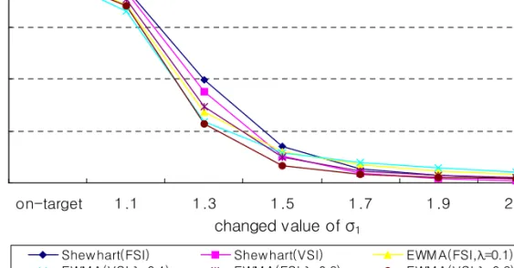
The properties and comparison of the proposed procedures are given in Table 5.1 through Table 5.3. From the numerical results, we found the following properties. VSI schemes are more efficient than FSI schemes in terms of ATS.
0 50 100 150 200
on-target 1.1 1.3 1.5 1.7 1.9 2.1
changed value of σ1
ATS values .
Shew hart(FSI) Shew hart(VSI) EWM A(FSI,λ=0.1) EWM A(VSI,λ=0.1) EWM A(FSI,λ=0.3) EWM A(VSI,λ=0.3)
Figure 5.1 ATS for the proposed charts (p = 3)
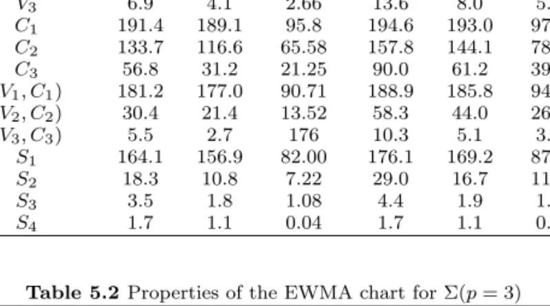
The results in Table 5.2 and Table 5.3 show that smaller smoothing constant λ is more efficient in detecting small shifts of the parameters in terms of ANSS and ATS.
And, we also found that the EWMA procedures exhibit far fewer switches when compared to the Shewhart procedure. Also, it was established that smaller values of λ for EWMA procedures will reduce the ANSW between two sampling intervals, respectively. The optimal selection of λ depends on the size of the shifts to be detected quickly.
p = 3 p = 4
types of shift ANSS ATS ANSW ANSS ATS ANSW
in-control 200.0 200.0 100.12 200.0 200.0 99.94 V1 186.2 183.2 93.24 192.3 190.2 96.09
V2 35.2 26.2 16.21 68.7 54.5 32.52
V3 6.9 4.1 2.66 13.6 8.0 5.38
C1 191.4 189.1 95.8 194.6 193.0 97.20
C2 133.7 116.6 65.58 157.8 144.1 78.19
C3 56.8 31.2 21.25 90.0 61.2 39.26
(V1, C1) 181.2 177.0 90.71 188.9 185.8 94.36 (V2, C2) 30.4 21.4 13.52 58.3 44.0 26.99
(V3, C3) 5.5 2.7 176 10.3 5.1 3.49
S1 164.1 156.9 82.00 176.1 169.2 87.88
S2 18.3 10.8 7.22 29.0 16.7 11.27
S3 3.5 1.8 1.08 4.4 1.9 1.21
S4 1.7 1.1 0.04 1.7 1.1 0.45
Table 5.2 Properties of the EWMA chart for Σ(p = 3)
λ = 0.1 λ = 0.2 λ = 0.3
types of shift ANSS ATS ANSS ANSS ATS ANSW ANSS ATS ANSW
in-control 200.0 200.0 27.46 200.1 200.0 40.48 200.0 200.0 50.29
V1 170.7 164.7 23.08 173.0 166.6 34.84 176.1 170.4 44.25
V2 29.5 29.0 3.26 24.9 18.6 4.21 24.8 16.5 5.34
V3 11.8 14.0 2.13 8.1 7.5 2.11 6.9 5.4 2.05
C1 178.8 174.1 24.24 181.3 176.4 36.64 183.9 179.6 46.21
C2 77.8 64.6 8.71 84.2 63.8 15.29 93.7 71.6 21.93
C3 24.4 23.7 2.48 21.3 13.6 2.89 23.3 11.3 3.58
(V1, C1) 157.9 150.4 21.10 162.8 154.3 32.70 167.4 159.6 41.97
(V2, C2) 25.9 26.1 2.92 21.2 15.9 3.57 20.9 13.6 4.39
(V3, C3) 9.7 11.7 2.02 6.5 6.2 1.95 5.5 4.3 1.82
S1 132.2 121.3 17.25 138.0 125.0 27.36 143.5 131.0 35.72
S2 18.0 19.6 2.38 13.5 10.8 2.56 12.7 8.2 2.78
S3 7.6 9.2 1.97 4.9 4.8 1.84 4.1 3.3 1.61
S4 4.4 5.4 1.76 2.9 2.8 1.39 2.3 1.9 1.03
Table 5.3 Properties of the EWMA chart for Σ(p = 4)
λ = 0.1 λ = 0.2 λ = 0.3
types of shift ANSS ATS ANSS ANSS ATS ANSW ANSS ATS ANSW
in-control 200.0 200.0 27.29 200.0 200.0 40.39 200.0 200.0 50.28
V1 181.1 177.0 24.49 184.0 179.5 37.03 186.0 181.9 46.71
V2 44.6 41.6 4.51 41.7 30.6 6.85 44.5 30.5 9.60
V3 17.7 20.8 2.32 12.5 11.2 2.46 11.2 8.2 2.63
C1 186.4 183.0 25.23 189.2 185.7 38.15 190.0 186.9 47.76
C2 104.0 89.9 12.34 113.9 93.6 21.54 123.4 102.8 29.73
C3 37.7 34.4 3.26 36.9 23.0 4.86 42.7 22.8 7.34
(V1, C1) 172.6 166.6 23.17 176.6 170.1 35.45 179.7 173.7 45.09
(V2, C2) 38.3 36.7 3.78 34.6 25.1 5.46 36.9 24.0 7.59
(V3, C3) 14.5 17.6 2.14 9.9 9.2 2.18 8.6 6.4 2.20
S1 142.4 131.9 18.50 149.5 136.9 29.65 155.6 143.6 38.73
S2 21.9 24.1 2.46 16.9 13.2 2.70 16.4 10.1 3.13
S3 9.4 12.0 2.01 6.0 6.1 1.97 4.9 4.1 1.85
S4 5.5 7.2 1.86 3.4 3.6 1.68 2.7 2.4 1.33
References
Alt, F. B. (1984). Multivariate quality control in the Encyclopedia of statistical sciences, Ed. S. Kotz and Johnson, John Wiley, New York.
Amin, R. W. and Letsinger, W. C. (1991). Improved swiching rules in control procedures using variable sampling intervals. Communications in Statistics- Simulation and Computation, 20, 205-230.
Chang, D. J., Kwon, Y. M. and Hong, Y. W. (2002). Markovian EWMA control chart for several quality characteristics. Journal of the Korean Data & Information Science Society, 14, 1045-1053.
Kwon, Y. M. and Chang, D. J. (2006). Evaluating properties of variable sampling interval EWMA control charts for mean vector. Journal of the Korean Data & Information Science Society, 16, 639-650.
Hotelling, H. (1947). Multivariate quality control, techniques of statistical analysis, McGraw-Hill, New York, 111-184.
Lucas, J. M. and Saccucci, M. S. (1990). Exponentially weighted moving average control schemes: Prop- erties and enhancements. Technometrics, 32, 1-12.
Reynolds, M. R., Jr. (1989). Optimal variable sampling interval control charts, Technical report 88-22, Virginia Polytechnic Institute and State University, Department of Statistics.
Reynolds, M. R., Jr., Amin, R. W. and Arnold, J. C. (1990). CUSUM charts with variable sampling intervals. Technometrics, 32, 371-384.
Vargas, V. C. C., Lopes, L. F. D. and Sauza, A. M. (2004). Comparative study of the performance of the CUSUM and EWMA control charts. Computer & Industrial Engineering, 46, 707-724.
Woodall, W. H. and Ncube, M. M. (1985). Multivariate CUSUM quality control procedure. Technometrics, 27, 285-292.