Analysis of Tilting Angle of KOMPSAT-1 EOC Image for Improvement of Geometric Accuracy Using Bundle Adjustment
Doochun Seo , Donghan Lee, Jongah Kim, Yongseung Kim
Satellite Operation & Application Center Korea Aerospace Research Institute P.O. Box 113, Yusung, Daejeon, 305-600 Phone: +82-42-860-2646 Fax: +82-42-860-2646
E-mail: {dcivil, dhlee, kja, yskim}@kari.re.kr
ABSTRACT
As the KOMPSAT-1 satellite can roll tilt up to
± 45
o, we have analyzed some EOC images taken at different tilt angles for this study. The required ground coordinates for bundle adjustment and geometric accuracy, are read from the digital map produced by the National Geography Institution, at a scale of 1:5,000.These are the steps taken for the tilting angle of KOMPSAT-1 satellite to be present in the evaluation of the accuracy of the geometric of each different stereo image data: Firstly, as the tilting angle is different in each image, the satellite dynamic characteristic must be determined by the sensor modeling. Then the best sensor modeling equation is determined.
The result of this research, the difference between the RMSE values of individual stereo images is due more the quality of image and ground coordinates than to the tilt angle. The bundle adjustment using three KOMPSAT-1 stereo pairs, first degree of polynomials for modeling the satellite position were sufficient.
Key words : Tilt angle, KOMPSAT-1 EOC, Position Accuracy, Bundle Adjustment
1. Introduction
Korea Multi-Purpose Sarellite-1(KOMPSAT-1) was successfully launched by Korea in 1999 and became one of the countries in the world to have their own earth observation satellites. KOMPSAT-1 is designed for multiple missions to provide various applications in the field of earth observation covering land and sea. Its main mission is for the production of Korea cartography. Images are collected and processed to support the development of maps of Korean Peninsula. EOC is KOMPSAT-1’s main payload for the purpose of cartography to produce digital map of Korea.
In this paper, we analyzed the geometric accuracy of KOMPSAT-1 EOC image, with can vary tilting angle conditions. As the KOMPSAT-1 satellite can roll tilt up to
± 45
o, we have analyzed some EOC images taken at three different tilt angles(5º, 15º, 27º) for this study. The required ground coordinates forbundle adjustment and geometric accuracy, are read from the digital map produced by the National Geography Institution, at a scale of 1:5,000 and the image coordinates are read with the sub-pixel accuracy.
These are the steps taken for the tilting angle of KOMPSAT-1 satellite for the evaluation of the accuracy of the geometric of each different stereo image data: Firstly, as the tilting angle is different in each image, the satellite dynamic characteristic must be determined by sensor modeling, and the best sensor modeling equation is determined. Then the control points (from the sensor modeling equation) are evaluated by calculating of the covariance matrix (
σ
X ,σ
Y,σ
XY,σ
Z) and image coordinates’ residual (V
X,V
Y) related to the ground coordinates. Finally, the check points are evaluated through RMSE’s coordinate of check points, which were calculated from sensor modeling.2. Bundle Adjustment for Linear Array CCD Sensor
The image data applied in this work is collected as follows. The satellite moves along a well defined close-to-circular elliptical orbit. Along track the sensor is always pointing to the center of the earth. The images are taken with pushbroom type, a constant time interval. The images taken have a cylindrical perspective, usually distorted due to attitude variations. A single image consists of a fixed number of consecutive scan lines. Each line has its own time-dependent position and attitude parameters. These exterior orientations are represented by 6 parameters. (3 parameters; position, 3 parameters; attitude) Behave these position and attitude parameters, due to correlation one part can become fixed.
The applied bundle adjustment utilized the orbital geometry in which orbital parameters are used to determine the satellite position and orientation with respect to the ground coordinates system at any time.
The actual position
S ( X
s, Y
s, Z
s)
of the satellite at a given time, deviates from the nominal positionS ′ ( X
s′ , Y
s′ , Z
s′ )
. These deviations are modeled as time polynomials to be included in the mathematical model in order to actual satellite positions and orientation. The actual satellite position can be calculated as follows:
∆
∆
∆ +
=
∆
∆
∆ +
′
′
′
=
′ Z
Y X
R M Z Y X
Z Y X
Z Y X
s T b s
s s
s s s
0 0
(1)
s b
R
M ,
can be calculated from the Eulerian parameters, which are also estimated using the ephemeris data. To determine the satellite orientation, the rotation matrixM
bis multiplied by another rotation matrixM
a. TheM
awill take care of angular deviations caused by the various unknown forces and the ellipsoidal figure of the earth.We can write the following set of collinearity equation for any point vector:
∆
∆
∆
−
−
=
′
′
′
′
Z
Y X
R M Z Y X M M k z y x M
s T b b
a
T
0
0
(2)
where,
M
Tis Tilt angle, the position deviation vector along the∆ X , ∆ Y , ∆ Z
direction are given by;2 2 1
0 X t X t
X
X = + ∆ + ∆
∆
δ δ δ
2 2 1
0 Y t Y t
Y
Y = + ∆ + ∆
∆
δ δ δ
(3)2 2 1
0 Z t Z t
Z
Z = + ∆ + ∆
∆
δ δ δ
The angular deviation around the three axes are modeled as time polynomial function similarly to that of above. The following is the evaluation of these angular deviations;
2 2 1
0+∆ ∆t+∆ ∆t
∆
=
∆
ω ω ω ω
2 2 1
0+∆ ∆t+∆ ∆t
∆
=
∆
φ φ φ φ
(4)2 2 1
0+∆ ∆t+∆ ∆t
∆
=
∆
κ κ κ κ
3. Data and Study Area
The EOC data used in this study includes three stereo images of KOMPSAT-1 digital images. We tested the KOMPSAT-1 tilting capability. The study area of these images are a stereo image in Daejeon area and two stereo images in Seoul area. These are level 1A images with ephemeris and attitude data recorded in panchromatic mode. At this level only detector normalization occurred, with no geometric correction for earth curvature or view angle effects applied.
Table 1. Specifications of the three stereo images
Pre-processing Level 1R Level 1R Level 1R Level 1R Level 1R Level 1R Scene Center Time 2001/04/08 2000/03/01 2001/11/27 2001/09/10 2000/03/09 2001/10/25
GRS K 927 928 927 927 928 927
GRS J 1324 1325 1334 1334 1334 1334
Orbit Number 6920 1032 10327 9186 1149 9844
Look Angle(deg.) -6.86 4.00 -15.29 15.25 -25.91 27.38
Orientation Angle (deg.) 10.01 10.02 -9.57 -14.37 10.16 -15.82
Solar Azimuth (deg.) 138.78 143.72 160.51 138.86 147.81 151.14
Solar Elevation (deg.) 54.22 39.03 29.06 50.52 43.04 35.82
Area Daejeon Seoul Seoul
Name Daejeonช Seoulช Seoulซ
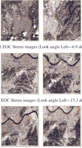
These stereo images are shown in Fig. 1, Fig. 2 and Fig. 3. This area contains cities, mountains and plains where the elevation ranges from 0 to about 700 m.
To apply bundle adjustment and verify the model fidelity, the 12 ground control points(GCPs) and about 10 check points(CKPs) distributed around the entire stereo image were selected. The 3D ground coordinates for GCPs and CKPs were captured by a CAD system from a 1:5,000-scale national digital maps in 1995. These captured rectangular planimetric coordinates and height on a geoid were transformed to the Earth-fixed Cartesian coordinates of the World Geodetic System 1984(WGS84) using the Bursa-Wolf model of 7-parameters and the EGM96 model.
The left image coordinates for GCPs and CKPs were determined from magnified images using ERDAS IMAGINE software system. The right image coordinates for GCPs and CKPs were determined using a GCP matching tool from the ERDAS IMAGINE software system. The test images, 12 GCPs marked with triangles and about 10 CKPs marked with circles are shown in Fig. 1, Fig. 2. and Fig 3.
Fig. 1. KOMPSAT-1 EOC Stereo images (Look angle Left=-6.9 deg., Right=4.0 deg.)
Fig. 2 . KOMPSAT-1 EOC Stereo images (Look angle Left=-15.3 deg., Right=15.2 deg.)
Fig. 3 KOMPSAT-1 EOC Stereo images (Look angle Left=-25.9 deg., Right=27.4 deg.)
4. Experiments and Results
These are the steps taken for the tilting angle of KOMPSAT-1 for in the evaluation of the accuracy of geometric of each different stereo image data: Firstly, as the tilting angle is different in each image, the satellite dynamic characteristic must be determined by sensor modeling and the best sensor modeling equation can be determined. Then the control points (from the sensor modeling equation) are evaluated by the calculation of the covariance matrix (
σ
X ,σ
Y,σ
XY,σ
Z ) and image coordinates’ residual (V
X ,V
Y) related to the ground coordinates. Finally, the check points are evaluated through RMSE’s coordinate of the check points, which were calculated from the sensor modeling.Several cases of experiments were tested to investigate the performance of the polynomial orders as a function of the satellite position deviations or angular deviations of Eq.(3) or (4). 12 GCPs and about 10 CKPs distributed around the entire stereo full scenes were used for tests of different orders for
Z Y X ∆ ∆
∆ , ,
and∆ ω , ∆ φ , ∆ κ
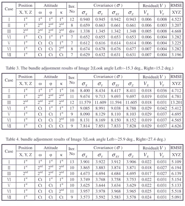
.Table 2. The bundle adjustment results of Image 1(Look angle Left=-6.9 deg., Right=4.0 deg.) Position Attitude Covariance (
σ
) Residual(V ) RMSE CaseX, Y, Z ω φ κ Iter.
No
σ
Xσ
Yσ
XYσ
ZV
XV
Y XYZช 1st 1st 1st 1st 12 0.940 0.945 0.942 0.943 0.006 0.008 4.523 ซ 1st 2nd 2nd 2nd 8 0.659 0.663 0.661 0.661 0.006 0.003 3.207 ฌ 2nd 2nd 2nd 2nd div 1.338 1.345 1.342 1.348 0.005 0.008 4.668 ฏ 1st Ct 1st 1st 7 0.652 0.655 0.653 0.653 0.006 0.004 3.282 ฎ 1st Ct Ct 1st 7 0.612 0.616 0.614 0.614 0.006 0.004 3.225 ฏ 1st Ct Ct 2nd 8 0.674 0.678 0.676 0.677 0.007 0.004 3.282 ฐ 1st Ct Ct Ct 7 0.629 0.632 0.631 0.631 0.007 0.004 3.196
Table 3. The bundle adjustment results of Image 2(Look angle Left=-15.3 deg., Right=15.2 deg.) Position Attitude Covariance (
σ
) Residual(V ) RMSE CaseX, Y, Z ω φ κ Iter.
No
σ
Xσ
Yσ
XYσ
ZV
XV
Y XYZช 1st 1st 1st 1st 16 8.400 8.434 8.417 8.411 0.018 0.036 4.712 ซ 1st 2nd 2nd 2nd 11 9.674 9.713 9.693 9.697 0.019 0.034 4.781 ฌ 2nd 2nd 2nd 2nd 12 11.579 11.609 11.594 11.605 0.018 0.031 13.201 ฏ 1st Ct 1st 1st 17 9.085 8.991 9.038 8.788 0.029 0.042 5.412 ฎ 1st Ct Ct 1st 9 8.090 8.129 8.110 8.103 0.029 0.037 4.695 ฏ 1st Ct Ct 2nd 10 8.131 8.169 8.150 8.152 0.019 0.037 4.565 ฐ 1st Ct Ct Ct 9 7.814 7.851 7.833 7.828 0.029 0.037 4.626
Table 4. bundle adjustment results of Image 3(Look angle Left=-25.9 deg., Right=27.4 deg.)
Position Attitude Covariance (
σ
) Residual(V ) RMSE CaseX, Y, Z ω φ κ Iter.
No
σ
Xσ
Yσ
XYσ
ZV
XV
Y XYZช 1st 1st 1st 1st 13 3.901 3.922 3.912 3.906 0.022 0.031 5.109 ซ 1st 2nd 2nd 2nd 10 3.865 3.883 3.874 3.871 0.018 0.027 6.194 ฌ 2nd 2nd 2nd 2nd 10 4.673 4.694 4.684 4.695 0.017 0.027 6.139 ฏ 1st Ct 1st 1st 10 3.749 3.768 3.758 3.753 0.022 0.031 5.154 ฎ 1st Ct Ct 1st 10 3.625 3.644 3.634 3.629 0.022 0.031 5.133 ฏ 1st Ct Ct 2nd 11 3.957 3.978 3.968 3.965 0.025 0.031 5.518 ฐ 1st Ct Ct Ct 9 3.573 3.592 3.583 3.578 0.024 0.031 5.091
5. Discussion
The RMSEs of Table 2, Table 3 and Table 4 provide some information on the differences between the function of polynomial order for the satellite position deviations or angular deviations. These three experiments are repeated at three different tilt angles of 5º, 15º and 25º, and the results are shown in Table 2, Table 3 and Table 4. Generally, the linear position models perform better than the quadratic model.
As the order of polynomial degrees increase, the adjusted ground coordinates of the standard deviation also increases. That is, rather than the bundle adjustment precision decreasing, polynomial order of
exterior orientation increase and the weighting factors also increases. As the tilt angle increase, the image coordinates residuals increase too. This is the conversion speed of bundle adjustment is unstable. In the process of bundle adjustment, most of the tests had been executed 10 times under. This shows the high speed of conversion iteration.
After bundle adjustment, by utilizing images of 3 different tilt angles, the results of sensor modeling;
The Daejeonชand Seoulซ of stereo pairs, the best case of adjusted parameters is case with results ฐ the other 6 cases. Case ฐ is first degree of polynomials with
∆ X , ∆ Y , ∆ Z
, constant forφ ω ∆
∆ ,
,∆κ
where average RMSE is 3.196 meters and 5.091 meters. In Seoulช stereo pair, the best case of adjusted parameters is case ฏ with results the other 6 cases. Case ฏ is first degree of polynomials with∆ X , ∆ Y , ∆ Z
, constant for∆ ω , ∆ φ
and quadratic ∆κ
where average RMSE is 4.565 meters.By looking at the check point accuracy in Table 2, 3 and 4 the average RMSEs(3.196m, 4.565m, 5.091m) are all 1 pixel below KOMPSAT-1 EOC spatial resolution. This does not greatly influence the tilt angle. The change in the tilt angle does not increase of the accuracy of ground object coordinates. The tilt angle effects two quality of image coordinates, especially since the image u-coordinates are sensitive.
This is because the tilt rotates around the u-axis. For the v-coordinates, the tilt increase does reduce the required error magnitude, and the same is true for the combined case.
6. Conclusions
The effect of the tilt angle on the mathematical model’s in exterior orientation parameters errors are studied in this research. These are the steps taken for the tilting angles (5º, 15º, 25º) of KOMPSAT-1 satellite for the evaluation of the accuracy of the geometric of three different stereo images: Firstly, as the tilting angle is different in each image, the satellite dynamic characteristic must be determined by sensor modeling. Then the best sensor modeling equation is determined. The best set of parameters are the 6 position deviation parameters with 1 yaw angle or three yaw angle deviation parameters in addition. The change in the tilt angle does not increase of the accuracy of the ground object coordinates. The change in the tilt angle does not increase of the accuracy of ground object coordinates. The tilt angle effects two quality of image coordinates, especially since the image u-coordinates are sensitive.
Reference
1. Makki, S. H. 1991, Photogrammetric reduction and analysis of real and simulated SPOT imageries, Purdue University, A thesis of Purdue University; 17-45.
2. E. M. Mikhail, J. S. bethel, 2001, Introduction to Modern Photogrammetry, New York, John Wiley and Sons Ins.
3. http://www.kari.re.kr