kfas

(1)

한수지 54(5), 769-781, 2021

769

Korean J Fish Aquat Sci 54(5),769-781,2021

Original Article

서 론

한국해역의살오징어(Todarodes pacificus)^는^다양한^어구를 통해어획되는대표적인복수어업대상종중하나이다. 현재총 41개의연근해어업중 21개어업에서살오징어를어획하고있 으며, 6^개^어업(^{근해채낚기}^어업, ^대형^트롤^어업, ^대형^선망^어 업, 동해구중형트롤어업, 근해자망어업, 그리고쌍끌이대형 저인망어업)이살오징어 TAC (total allowable catch) 대상어

업에참여하고있다. 그런데 2000년대초반이후로한국해역의

살오징어연간어획량은크게감소하고있는실정이다. 2003년

약 23^만톤에^이르던^살오징어^어획량이 2015^년에는^약 15^만톤 으로급격히감소하였으며이후, 지속적인감소를거쳐 2018년 의어획량이약 4만톤으로기록된사실은살오징어자원의심

각성을시사하는바이다(KOSTAT, 2020). ^하지만^이러한^상황

에도불구하고살오징어자원평가에대한연구는현재까지부 재한상황이다. 현존하는수집자료(e.g., 연령자료, 직접자원조 사자료, 등)도단기간에국한되어있거나부재하며, 단일어업 이아닌복수어업을고려한자원평가연구가상당히제한적인 상황이다. ^이런^상황^속에서^{살오징어를}^어획하는^여러^어업들 의 CPUE (catch per unit effort)자료가수집되었다는점은잉여 생산량모델의적용가능성과복수어업을고려한자원평가의 활용가능성을제시한다. 현재까지잉여생산량모델을적용한 대부분의자원평가연구를살펴보면단일어업의 CPUE자료만 을이용하여자원평가를수행했다(Hilborn and Walters, 1992;

Millar and Meyer, 2000; Punt and Szuwaiski, 2021; Hyun and

Kim, 2022). 하지만실제로는여러어업에서어느한개체군을

한국 해역의 살오징어(Todarodes pacificus) 개체군 자원평가를 위한 베이지안 상태공간 잉여생산량 모델의 적용

안동영·김규한¹·강희중²·현상윤*

부경대학교 해양생물학과, ¹웰링턴 빅토리아대학교 수학 통계학부, ²국립수산과학원 연근해자원과

A Bayesian State-space Production Assessment Model for Common Squid Todarodes pacificus Stock Caught by Multiple Fisheries in Korean Waters

Dongyoung An, Kyuhan Kim¹, Heejung Kang² and Saang-Yoon Hyun*

College of Fisheries Sciences, Pukyong National University, Busan 48513, Korea

1School of Mathematics and Statistics, Victoria University of Wellington, Wellington 6140, New Zealand

2Coastal Water Fisheries Resources Research Division, National Institute of Fisheries Science, Busan 46083, Korea

Given data about the annual fishery yield of the common squid Todarodes pacificus, and the catch-per-unit-effort (CPUE) data from multiple fisheries from 2000-2018, we applied a Bayesian state - space assessment model for the squid population. One of our objectives was to do a stock assessment, simultaneously incorporating CPUE data from the following three fisheries, (i) large trawl, (ii) jigger, and (iii) large purse seine, which comprised on average a year about 65% of all fisheries, allowing possible correlations to be reflected. Other objectives were to consider both observation and process errors and to apply objective priors of parameters. The estimated annual exploitable biomass was in the range of 3.50×10⁵ to 1.22×10⁶ MT, the estimated intrinsic growth rate was 1.02, and the estimated carry- ing capacity was 1,151,259 MT. Comparison with available results from stock assessment of independently analyzed single fisheries revealed a large difference from the estimated values, suggesting that stock assessment based on multiple fisheries should be performed.

Keywords: Todarodespacificus, Multiple fisheries, Bayesian state space Schaefer model, TMB

*Corresponding author: Tel: +82. 51. 629. 5929 Fax: +82. 51. 629. 5931 E-mail address: [email protected]

This is an Open Access article distributed under the terms of the Creative Commons Attribution Non-Commercial Licens (http://creativecommons.org/licenses/by-nc/3.0/) which permits unrestricted non-commercial use, distribution, and reproduction in any medium, provided the original work is properly cited.

Received 1 July 2021; Revised 20 July 2021; Accepted 12 August 2021

저자 직위: 안동영(대학원생), 김규한(대학원생), 강희중(연구사), 현상윤(교 수)

https://doi.org/10.5657/KFAS.2021.0769

Korean J Fish Aquat Sci 54(5), 769-781, October 2021

(2)

어획하기때문에복수어업을고려한자원평가연구가필요하 다(Pascoe et al., 2020). 이런상황속에서최근에잉여생산량 모델을바탕으로복수어업을고려한자원평가연구가소개된 바있다(Hyun, 2018; Winker et al., 2020). 하지만 Hyun (2018)

에서는자원량의과정오차를별도로고려하지않았고, Winker

et al. (2020)^의^경우, ^여러^어업의 CPUE^를^서로^독립으로^가정 하였으며, 어업선택성을반영하였으나입력값으로고려했다 는단점을지니고있다.

따라서본연구는크게두가지목적에기반을두고있다. 첫째 로는베이지안상태공간잉여생산량모델에복수어업을고려 한살오징어개체군자원평가를실시하는것이다. ^둘째로는^복 수어업을고려했을때와단일어업만을고려했을때의자원평가 결과를비교및분석하여복수어업을고려한자원평가의필요 성을증명하는것이다. 본연구에서는기존잉여생산량모델에 상태공간구조를적용함으로써추정하고자하는자원량의과정 오차와자료의관측오차를동시에고려하였다. ^그리고^여러^어

업의 CPUE자료가다변량정규분포를따른다고가정하며복수

어업 CPUE간의상관관계를추가적으로고려하였다. 그런데

TMB R package를바탕으로상태공간잉여생산량모델을적

용했을때수치최적화가제대로이루어지지않았기때문에본 연구에서는정보적사전분포를바탕으로베이지안방법론을적 용하였다. 그리고한국해역의살오징어의경우, 어업선택성에 관한정보가부재한상황이다. 국립수산과학원으로부터제공

받은여러어업의 CPUE자료는상업어업으로부터수집된자

료이며본연구에서는어업선택성을별도로고려하지않았다. 베이지안상태공간잉여생산량모델을적용한한국해역의살 오징어자원평가는두가지방식으로실시하였다. 첫번째는복 수어업을고려한방식으로써세가지어업의 CPUE자료를베 이지안상태공간잉여생산량모델에적용하여모수를추정하였 다(이하 Case I). 두번째는단일어업만을고려한방식으로써각

어업별하나의 CPUE^자료를^베이지안^상태공간^{잉여생산량}^모

델에적용하여모수를추정하였다(이하 Case II). Case II의경 우적용하는단일어업에따라 3개의케이스(case)로다시구분 하였다: i) 근해채낚기어업만을고려한방식(이하 Case II-1), ii) 대형선망어업만을고려한방식(이하 Case II-2), 그리고 iii) 대형트롤어업만을고려한방식(^이하 Case II-3). ^베이지안^상 태공간잉여생산량모델을바탕으로복수어업을고려한살오징

어자원평가(Case I)를주요결과로서도출하였으며복수어업

을고려한경우(Case I)와단일어업만을고려한경우(Case II) 의자원평가결과를비교해보았다.

재료 및 방법

살오징어 자료

통계청에서 2000년부터 2018년까지수집한한국해역의연도

별살오징어총어획량자료(KOSTAT, 2020)^와^동기간의^국

립수산과학원에서수집한 CPUE^자료를^본^연구에^{이용하였다}. 한국해역에서살오징어를어획하는세가지어업의 CPUE자 료를사용하였으며, 구체적으로 2000년부터 2018년까지살오 징어총어획량의약 33.5%를차지하는대형트롤(large trawl, tw) ^어업과^약 27.3%를차지하는근해채낚기(jigger, jig) ^어업, 그리고약 4.2%^를^차지하는^대형선망(large purse seine, ps) ^어

업의 CPUE자료를사용하였다. 해당세종류의어업만을고려

한이유는해당어업이 2018년을기준으로살오징어 TAC 대

상어업에참여하고있음과동시에 CPUE자료의수집이가능

하였기때문이다.

본연구의대상종인살오징어는우리나라전체해역, ^동중국 해, 그리고일본북해도이남까지북서태평양전체를대상시 스템으로분포하고있다. 하지만본연구에서는한국해역에서

수집한어획량, CPUE자료만을연구에이용하였기때문에대

상해역을한국해역으로한정하였다. 그리고국립수산과학원

에서수집한여러어업의 CPUE^자료에는^조업^해역에^대한^정

보, 그리고어업선택성에대한정보가부재하기때문에어업 별살오징어에대한공간영역을우리나라의전체해역으로가 정하였다.

국립수산과학원에서수집한 CPUE (근해채낚기 CPUE, 대형

선망 CPUE, ^대형트롤 CPUE)^자료는^{직접자원조사자료가}^아

닌상업어업으로부터수집된자료이기때문에상대적개체군

의크기를나타내는 CPUE의단위와추세가어업마다서로상

이함을볼수있다(Fig. 1b-1c).

상태공간 잉여생산량모델

본연구에서는다양한형태의잉여생산량함수중, Schaefer 함수(Schaefer, 1954)를적용하였다. Pella and Tomlinson함수 (Pella and Tomlinson, 1969)도있지만, 모수를하나더추정해 야한다는단점이있기에 Schaefer함수를적용하였다. 그리고 기존잉여생산량모델에상태공간 구조를적용함으로써, 자료 의관측오차와자원량의과정오차를동시에고려하였다.

B₁=bKexp(ε₁^p ), where ε₁^p ~ N(0,σ_p²) ………… (1)

B_t+1=[B_t+B_t (1-BK_t)r-Y_t ]exp(ε_t+1^p),

where ε_t+1^p ~ N(0,σ_p²), and t ≥1………… (2) I_t=qB_t exp(ε_t^o ), where ε_t^o ~ N(0,σ_o² )………… (3)

여기서 t^는^연도, Y_t^는^연도별^어획량, I_t^는^연도별^상대적^개체 군크기, r^은^본원적^성장률, K^는^최대^{환경수용력}, b^는^초기^어 획가능자원량에최대환경수용력을나눈계수, ε_t^p는과정오차, ε_t^o는관측오차, q^는^{어획능률계수}, B_t^는^연도별^어획가능^자원

량을의미한다. 본연구에서사용하는연도별 CPUE자료는상

업어업에서수집된자료이며어업선택성이반영된자료이기

(3)

한국해역의 살오징어 개체군 자원평가 771

때문에 B_t^를^연도별^총^자원량이^아닌, 연도별어획가능자원량 으로정의하였다. 연도별 CPUE자료 I_t와연도별어획가능자원 량 B_t^는 q ^상수에^대하여^{비례관계를}^가진다.

본 연구에서 이용된 모든 표기기호에 대한 자세한 설명은

Table 1에별도로정리하였으며, 몇가지가정을기반으로모델

을표기하였다. 우선과정오차와관측오차가정규분포를따르 며평균이 0이고, 분산이각각 σ_p², σ_o²를가진다고가정하였다. 그리고, 수치최적화모수추정을위해과정오차의분산과관측 오차의분산이서로동일한값(σ_p²=σ_o²)^을^가지도록^{가정하였다} (Auger-Méthé et al., 2016). 식 (1)-(2)에서는 과정오차를고 려함으로써B_t^를^고정^모수가^아닌, 상태변수로가정하였다. 초 기어획가능자원량 B₁의경우, 식 (1)과같이상수 b에최대환 경수용력 K^와^함께^과정^오차를^고려한^{상태변수로}^가정하였 다. ^식 (3)^과^같이 CPUE^자료는^어획가능^자원량 B_t^에^비례하 며관측오차를추가적으로고려하였다(Polacheck et al., 1993;

Winker et al., 2018).

복수어업을 고려한 베이지안 상태공간 잉여생산량 모델 (Case I)

Case I^은 ^{복수어업을} ^고려한 ^{방식으로써}, ^세 ^가지 ^어업의

CPUE자료를이용하여베이지안상태공간잉여생산량모델에

적용한방식이다. 식 (1)-(3)에서의가정을동일하게유지하며

과정방정식과관측방정식을다음과같이표기하였다. B₁=bKexp(ε₁^p ), where ε₁^p ~ N(0,σ_p²) ………… (4)

B_t+1=[B_t+B_t (1-B_t/K)r-Y_t^total ]exp(ε_t+1^p),

where ε_t+1^p ~ N(0,σ_p²), and t ≥1 ………… (5) I_f,t=q_f B_t exp(ε_t^f ), where ε_t^f ~ N(0,σ_f² ) ………… (6)

여기서 f는어업의종류, Y_t^total는모든어업에서의살오징어연

도별총어획량, ε_t^f는각어업별 CPUE 자료의관측오차, q_f^는^각 어업별어획능률계수를의미한다.

살오징어총어획량자료와세가지어업의 CPUE자료를이용 하여어업선택성이반영된어획가능자원량 B_t^를^{추정하였다}. 식 (6)과같이각어업별 CPUE는B_t에직접비례하며각각의어 획능률계수 q_f^와^관측오차 ε_t^f를가진다고가정하였다. 세가지 어업의상관성을추가적으로고려하고자각어업별 CPUE^자료 를확률벡터로서고려하며다변량정규분포를따른다고가정하 였다. 수치최적화및모수추정을위해과정오차의분산과각 어업별관측오차의분산이동일한값(σ_p²=σ_f²)을가진다고가정 하였다(Auger-Méthé et al., 2016).

상태변수 B_t^의^단위를^낮추면서^{수치최적화의}^안정성을^향상 시키기위해 B_t^를^최대^{환경수용력} K^로^나누었다(P_t=B_t/K). ^그 리고양변에 log를취함으로써 logP₁, logP_t^가^다음의^식 (7), (8) 과같이정규분포를따르도록식을재구성하였다. 그리고각어

업별 CPUE 자료의경우식 (9)와같이확률벡터로서고려하며

다변량정규분포를따른다고가정하였다.

logP₁~N(log(b),σ_p² ) ………(7) Fig. 1. Annual yield of the common squid from 2000 to 2018 (panel a), the jigger fishery CPUE (dashed line with dots in panel b), the purse seine fishery CPUE (dashed line with open circles in panel b), and the trawl fishery CPUE (dashed line with open circles in panel c).

(4)

logP_t+1~N(log[P_t+rP_t (1-P_t )-Y_t/K],σ_p² ),

where t ≥1………… (8) I~N(u,∑), where I=(log(I_jig,t),log(I_ps,t),log(I_tw,t))^………(9) 식 (9)에서아래첨자 jig, ps, tw은각각근해채낚기어업, 대형 선망어업, 대형트롤어업을의미한다. 다변량정규분포의평균

은식 (10)^과^같이^{표기하였으며}, ^각^어업별^{상관계수를}^고려한

분산공분산행렬은다음의식 (11)와같이표기하였다.

u=(log(q_jigKP_t), log(q_psKP_t), log(q_twKP_t)) ……… (10)

∑=[σ^σ_jig^jig σ^σ^σ_tw^ps^jig^ρ ρ²^jig,ps_jig,tw

σ_jig σ_ps ρ_jig,ps σ_ps² σ_ps σ_tw ρ_ps,tw

σ_jig σ_tw ρ_jig,tw σ_ps σ_tw ρ_ps,tw

σ_tw² ]^…… ⁽¹¹⁾

분산공분산행렬중, 어업별상관계수 ρ_jig,ps, ρ_jig,tw, ρ_ps,tw는표

준화한어업별 CPUE자료를기반으로입력값으로써고려하였

다. 그값은각각 ρ_jig,ps=0.473 (P<.000), ρ_jig,tw=0.208 (P<.000), ρ_ps,tw=0.767 (P<.000)이다.

사전 분포

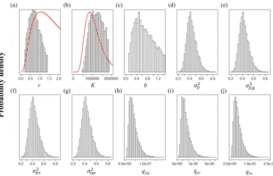
상태공간잉여생산량모델을적용했을때수치최적화가제대 로이루어지지않았기때문에정보적사전분포를바탕으로베 이지안방법론을도입하였다. 본연구에서는추정하고자하는 모수중, 본원적성장률 r과최대환경수용력 K에정보적사전 분포를적용하였다. Froese et al. (2017)에서는 FishBase의자 원회복력(resilience) ^정보를^활용하여^모수 r^과 K^에^정보적^사 전분포를주는방법을고안하였는데, Froese et al. (2017)의방 법을적용하여모수 r^과 K^에^정보적^{사전분포를}^적용했다. 한국 해역의살오징어는자원회복력이높은종으로써 FishBase의 자원회복력은 high로표시되어있다. 이정보를바탕으로 r^과 K 모수에정보적사전분포를설정할수있었다(Table 2). ^모수 r 과 K^가^로그^{정규분포를}^따른다고^{가정하였으며}, Froese et al.

(2017)에서의방법을활용하여각각의최빈값을 1.06, 855,264 로적용하였다. 그리고사전분포불확실성을낮추기위해변동 계수(coefficient of variation)는 1.0 (=100%)으로고려하였다. 그외, ^나머지^모수에는^무정보적^{사전분포를}^적용했다.

본논문에서적용한사전분포를독립으로가정하여결합사 전분포(joint prior distribution)를다음의식 (12)와같이표현 하였다.

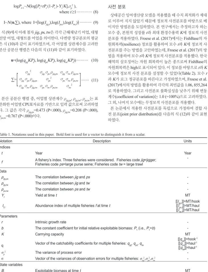
Table 1. Notations used in this paper. Bold font is used for a vector to distinguish it from a scalar.

Notation Description Units

Indices

t Year Year

f A fishery’s index. Three fisheries were considered. Fisheries code jig=jigger;

Fisheries code ps=large purse seine; Fisheries code tw = large trawl

-

Data

ρ_jig_,_ps The correlation between jig and ps -

ρ_jig_,_tw The correlation between jig and tw -

ρ_ps_,_tw The correlation between ps and tw -

Y_t Yield at time t MT

I_f_,_t Abundance index of multiple fisheries f at time t [[I_jig_,_t]]=MT/hook

[[I_ps_,_t]]=MT/haul [[I_tw_,_t]]=MT/haul Parameters

r Intrinsic growth rate -

b The constant coefficient for initial relative exploitable biomass: P₁ (i.e., P₁=b) -

K Carrrying capacity MT

q Vector of the catchability coefficients for multiple fisheries: q_jig, q_ps, q_tw [[q_jig]]=hook^-1 [[q_ps]]=haul^-1 [[q_tw]]=haul^-1

σ_p² The variance of process error -

σ Vector of the variances of observation errors for multiple fisheries: σ_jig²,σ_ps²,σ_tw² - State variables

B_t Exploitable biomass at time t MT

(5)

한국해역의 살오징어 개체군 자원평가 773

Pr(r,K)=Pr(r)Pr(K)……… (12)

우도 함수와 베이지안 방법론

과정오차 방정식과 관측오차방정식에 대한우도함수가상 호독립으로가정하며다음의식 (13), (14)^과^같이^{표시하였다}.

L(b,K,σ_p²,r,P│Y )= 12πσ_p exp[^{- (logP}²⁰⁰⁰_2σ^{-log(b) )}²

p2 ]

×²⁰¹⁸ 1 2πσ_p

∏

2000

exp[^-^(logP^t+1^-log[P^t_2σ^+rP^t^(1-P^t^)-Y^{K ])}^t ²

p ]^……⁽¹³⁾

L(q_jig,q_ps,q_tw,K,σ_jig²,σ_ps²,σ_tw²,P│ρ_jig,ps,ρ_jig,tw,ρ_ps,tw,I)=

×²⁰¹⁸∏(2π)^{- 3}²

2000 |∑|^{- 1}² exp[- 1

2 (I-u)^' ∑^-1(I-u)]……(14) 여기서, Y=(Y₂₀₀₀, Y₂₀₀₁, …, Y₂₀₁₈), 그리고 I=(log(I_jig,t), log(I_ps,t), log(I_tw,t))이다.

식 (13)는과정방정식의모수(b,r,K,σ_p²,P)를추정하기위한우 도함수, 식 (14)는관측방정식의모수(q_jig,q_ps,q_tw,K,σ_jig²,σ_ps²,σ_tw² ,P)^를^추정하기^위한^우도^함수이다. ^우도^함수에^대한^식 (13), (14)의결합우도함수(joint likelihood function)는다음의식 (15)와같다.

L(b,K,r,q_jig,q_ps,q_tw,σ_jig²,σ_ps²,σ_tw²,σ_p²,P│ρ_jig,ps,ρ_jig,tw ,ρ_ps,tw,I,Y)=

L(b,K,σ_p²,r,P│Y)·L(q_jig,q_ps,q_tw,K,σ_jig²,σ_ps²,σ_tw²,P

│ρ_jig,ps,ρ_jig,tw,ρ_ps,tw,I) …… (15)

식 (16)과같이결합사후분포는베이즈정리에따라결합사

전분포와결합우도함수에비례한다.

L(θ│ρ_jig,ps,ρ_jig,tw,ρ_ps,tw,I,Y)∝∫f (P,I,Y | θ) ·Pr(r,K)dP … (16) TMB와 상호 연동되는 tmbstan R package를 이용하여 MCMC (markov chain monte carlo) ^샘플링을^{실시하였으며},

Table 2. Prior probability density functions (PDFs) on parameters

Parameters Form of the prior Mode CV

r Log-normal (0.74, 0.69) 1.06 1.0 (=100%) K Log-normal (14.35, 0.69) 855,264 1.0 (=100%)

b Non-informative

σ_p² Non-informative

σ_jig² Non-informative

σ_ps² Non-informative

σ_tw² Non-informative

q_jig Non-informative

q_ps Non-informative

q_tw Non-informative

Note: CV, coefficient of variation.

Fig. 2. Posterior distributions of the respective parameters under Case I. The curve in panel a indicates the informative prior of r, and that in panel b represents the informative prior of K.

(6)

총 3,000,000^개의^표본을^{추출하였다}. ^이^중^초기 15,000^개의

표본을번인(burn-in) 처리하였으며추출된표본간의자기상

관(auto correlation)을제거하기위해매 100번째표본을추출 하였다(thinning). 그결과, 총 15,000개의표본을이용하여사 후분포를형성하였다.

추정하고자하는모수(b,r,K,q_jig,q_ps,q_tw,σ_jig²,σ_ps²,σ_tw² σ_p²)^의^사후 분포가형성된후, 사후분포의수렴여부및자기상관의정도를 진단하는과정을실시하였다. 본연구에서는 3가지방법을바 탕으로사후분포의수렴여부및자기상관의정도를진단하였 다(Hyun et al., 2005): (i) 라프테리와루이스통계(Raftery and

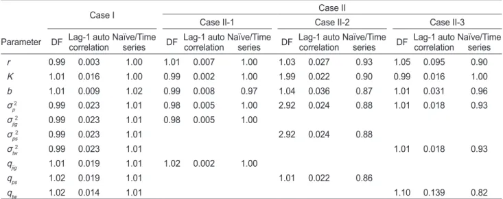
Table 3. Diagnostic tests for Markov Chain Monte Carlo samples for parameters (b,r,K,σ_p²,σ_jig²,σ_ps²,σ_tw², q_jig, q_ps, q_tw) from four different cases:

Case I (when multiple fisheries CPUE data were used), Case II-1 (when only jigger fishery CPUE data were used), Case II-2 (when only large purse seine fishery CPUE data were used), Case II-3 (when only large trawl fishery CPUE data were used

Case I Case II

Case II-1 Case II-2 Case II-3

Parameter DF Lag-1 auto correlationNaïve/Time

series DF Lag-1 auto correlationNaïve/Time

series DF Lag-1 autocorrelationNaïve/Time series

r 0.99 0.003 1.00 1.01 0.007 1.00 1.03 0.027 0.93 1.05 0.095 0.90

K 1.01 0.016 1.00 0.99 0.002 1.00 1.99 0.022 0.90 0.99 0.016 1.00

b 1.01 0.009 1.02 0.99 0.008 0.97 1.04 0.036 0.87 1.01 0.031 0.96

σ_p² 0.99 0.023 1.01 0.98 0.005 1.00 2.92 0.024 0.88 1.01 0.018 0.93

σ_jig² 0.99 0.023 1.01 0.98 0.005 1.00

σ_ps² 0.99 0.023 1.01 2.92 0.024 0.88

σ_tw² 0.99 0.023 1.01 1.01 0.018 0.93

q_jig 1.01 0.019 1.01 1.02 0.002 1.00

q_ps 1.02 0.019 1.01 1.01 0.022 0.86

q_tw 1.02 0.014 1.01 1.10 0.139 0.82

The dependence factor of Raftery-Lewies statistics (DF), lag-1 autocorrelation, and the ratio of the naïve standard error to the time series standard error were checked.

Table 4. Point estimates of parameters and their 95% credible intervals from four different cases

Parameters Case I Case IIh

Case II-1 Case II-2 Case II-3

r 1.02 (0.26, 1.32) 0.42 (0.21, 0.78) 0.74 (0.21, 0.81) 0.58 (0.17, 0.84)

K 1.15×10⁶

(6.46×10⁵, 1.82×10⁶) 1.57×10⁶

(9.29×10⁵, 1.84×10⁶) 8.17×10⁵

(7.23×10⁵, 1.78×10⁶) 1.12×10⁶ (7.73×10⁵, 1.83×10⁶)

b 0.99 (0.16, 1.88) 1.99 (1.07, 2.84) 1.11 (0.78, 2.84) 0.55 (0.11, 0.99)

σ_p² 0.41 (0.29, 0.63) 0.03 (0.02, 0.07) 0.10 (0.06, 0.28) 0.10 (0.06, 0.27)

σ_jig² 0.41 (0.29, 0.63) 0.03 (0.02, 0.07)

σ_ps² 0.41 (0.29, 0.63) 0.10 (0.06, 0.28)

σ_tw² 0.41 (0.29, 0.63) 0.10 (0.06, 0.27)

q_jig 3.29×10^-8

(1.58×10^-8, 9.78×10^-8) 2.59×10^-8 (1.71×10^-8, 6.05×10^-8)

q_ps 1.23×10^-6

(5.82×10^-7, 3.61×10^-6) 2.98×10^-6

(6.59×10^-7, 3.17×10^-6)

q_tw 3.19×10^-6

(1.51×10^-6, 9.39×10^-6) 4.12×10^-6

(1.14×10^-6, 6.02×10^-6) Case I (when multiple fisheries CPUE data were used), Case II-1 (when only jigger fishery CPUE data were used), Case II-2 (when only large purse seine fishery CPUE data were used), Case II-3 (when only large trawl fishery CPUE data were used). The 95% credible intervals of estimates are provided in parentheses, respectively.