Three-dimensional Computational Modeling and Simulation of Intergranular Corrosion Propagation of Stainless Steel
T. Igarashi
†, A. Komatsu, T. Motooka, F. Ueno, and M. Yamamoto
Japan Atomic Energy Agency, Tokai, Ibaraki 319-1195, Japan
(Received January 02, 2020; Revised February 26, 2021; Accepted February 26, 2021)
In oxidizing nitric acid solutions, stainless steel undergoes intergranular corrosion accompanied by grain dropping and changes in the corrosion rate. For the safe operation of reprocessing plants, this mechanism should be understood. In this study, we constructed a three-dimensional computational model using a cel- lular automata method to simulate the intergranular corrosion propagation of stainless steel. The compu- tational model was constructed of three types of cells: grain (bulk), grain boundary (GB), and solution cells. Model simulations verified the relationship between surface roughness during corrosion and disper- sion of the dissolution rate of the GB. The relationship was investigated by simulation applying a constant dissolution rate and a distributed dissolution rate of the GB cells. The distribution of the dissolution rate of the GB cells was derived from the intergranular corrosion depth obtained by corrosion tests. The constant dissolution rate of the GB was derived from the average dissolution rate. Surface roughness calculated by the distributed dissolution rates of the GBs of the model was greater than the constant dissolution rates of the GBs. The cross-sectional images obtained were comparable to the corrosion test results. These results indicate that the surface roughness during corrosion is associated with the distribution of the corrosion rate.
Keywords: Intergranular corrosion, Stainless steel, Corrosion shape, Computer simulation, Cellular automata method
1. Introduction
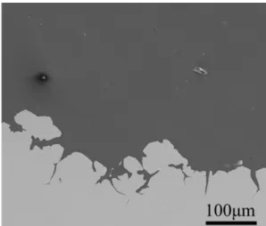
In spent fuel reprocessing plant, the corrosion of the components treating oxidizing nitric acid solution such as vessels, tanks and pipes is an important issue. It is known that austenitic stainless steel in oxidizing nitric acid solution is in transpassive state showing morphology of intergranular corrosion [1]. Fig. 1 shows a cross sectional image of austenitic stainless steel stayed in transpassive state of oxidizing nitric acid. The intergranular corrosion behaviour in oxidizing nitric acid solution gives grain dropping resulting a high corrosion rate [2]. The inter- granular corrosion was caused by presence of minor elements (e.g. C, P, S) in stainless steel. Especially, segregated C, P and S at GB could promote intergranular corrosion [3-6].
For safety operation of spent fuel reprocessing plants treating oxidizing nitric acid solutions, it is important to understand intergranular corrosion mechanism. For under-
standing intergranular corrosion mechanism, some researchers had developed computational model. Ohno et al. had developed the intergranular corrosion model considering cylindrical-shaped grains, and simulated the weight loss behaviour at the progressing intergranular corrosion [7].
Bague et al. had determined the penetration depth using GB dissolution model [8]. These studies showed comparable
†Corresponding author: [email protected]
T. Igarashi: Professor, A. Komatsu: Professor, T. Motooka:
Professor, F. Ueno: Professor, M. Yamamoto: Professor
Fig. 1. Cross-sectional image of stainless steel in transpassive state
stainless steel in oxidizing nitric acid solution. In the simulations, we considered distribution of dissolution rate at GBs caused by minor elements and clarified the relation between surface roughness and dissolution rate at GBs.
2. simulation model for intergranular corrosion
In our previous study, novel two dimensional inter- granular corrosion model was developed and the model suggested that various morphology of corrosion could simulate [9]. In this study, we extended our two dimensional model into three dimensional model using cellular automata method, and the simulation for intergranular corrosion was conducted using the extended model.
The cellular automata method is a discrete model which consists of a regular grid of cells, each in one of a finite number of states [10]. In this model, three dimensional space was parted into small cells. Three cells were set:
interior of grain (bulk) cell, GB cell, and solution cell.
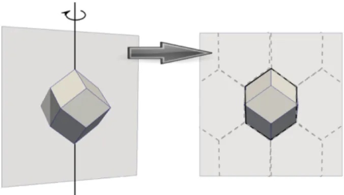
The only bulk and/or GB cell contacted with solution cell corrode and change into solution cells. The shape of cell was set to rhombic dodecahedron [11] as shown in Fig.
2. The rhombic dodecahedron is a convex polyhedron with 12 congruent rhombic faces, and this tessellation can be seen as the Voronoi tessellation of the face-centered cubic lattice. Schematic example of simulation of
to give us flexibility of making various shapes of grains.
The ratio of rate for changing to solution cell from bulk cell, vbulk, and GB cell, vGB, was defined in equation (1).
(1) LGB and Lbulk are corrosion depth and penetration depth respectively as shown in Fig. 4.
Corrosion progressing length rbulk/GB was defined as follows:
(2) where Δt represents time step of the simulation.
During the simulation, if rbulk/GB of each cell became larger than the length between central point of neighboured cells, rcell, bulk or GB cell changed into solution cell.
(3)
( )
bulk bulk GB bulk
GB
L L L v
v = +
∑ Δ
=
t
t v
r
bulk/GB bulk/GBcell bulk/GB
r r >
Fig. 2. Rhombic dodecahedron type cell
Fig. 3. Schematic example of simulation of corrosion progress; Corrosion is progressed from (a) to (c)
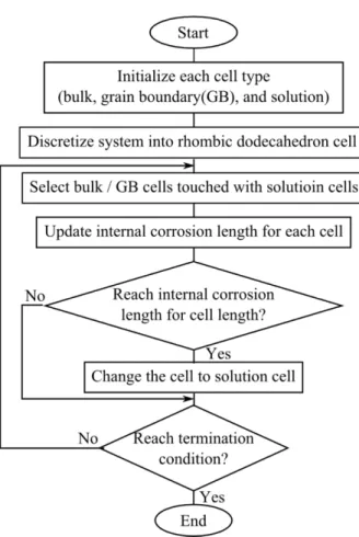
In this model, the surfaces are allowed to move for Δt by changing cells using equation (2) and (3), and corrosion is represented from macroscopic viewpoint. Fig. 5 represents flowchart of the simulation model.
In this study, the simulation system was constructed by a cube of 300 × 300 × 300 μm, and rcell length was / 2 μm. The mean grain size in the simulation was 50 μm
by setting positions of kernel points in Voronoi tessellation.
The dissolution rate of bulk cell was 2.0 × 10⁻¹⁰ m/s: this was derived from experimental corrosion test [13]. Δt must be set to satisfy the Courant-Friedrichs-Lewy (CFL) condition [14]. The CFL condition is a necessary condition for stability while solving certain partial differential equations numerically.
(4)
In order to make the simulation precisely, Δt was set as follows.
(5) Simulation for intergranular corrosion was performed and ended over 150 μm of thinning. The average and maximum corrosion depths were analysed after the simulation. The average corrosion depth was calculated by the weight loss of the simulation system. The maximum corrosion depth was the deepest point from original surface. These corrosion depths are shown in Fig. 6. The data set was discussed in section 3. The model in this study was own program and developed by C-language.
The ParaView software was used to visualize the cross- sectional and quarter view of intergranular corrosion simulation results [15].
3. data set for simulation
3.1 Distribution of intergranular corrosion rate Data set used for simulation was the distribution of dissolution rate at GBs. This is expressed in equation (6) as a probability density function:
2
cell
v
GBr > t Δ
GB cell
10v t = r Δ
Fig. 4. Schematic view of corrosion depth
Fig. 5. Flowchart of the intergranular corrosion simulation model
Fig. 6. Schematic view of average corrosion depth and maximum corrosion depth
vGB is average value which is calculated the data from our previous paper [13]. The corrosion test provided in our previous paper was presented in next subsection.
3.2 Corrosion test 3.2.1 material
One test material was Type310 stainless steel with extra high purity (Type310EHP stainless steel) [17,18]. It contains minor impurities such as C, P, S, and N: total concentration is less than 100 ppm. Other test material was Type310EHP having 270 ppm of phosphorus (Type 310-270P). It was thermal aged at 650oC or 24 hours to segregate P at GB. Table 1 shows chemical composition of the materials.
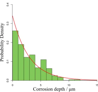
The specimen was dissolved by constant polarization at 1.1 V vs SSE. Volume of dissolved specimen was controlled by electric charge of 5 × 10⁴C/m2. In this condition, mean penetration depth Lbulk was about 1μm.
The corrosion depth LGB was measured using cross- sectional SEM images.
4. Results and Discussion
4.1 Cross-sectional images and quarter view
Fig. 8 shows cross-sectional images of intergranular
Fig. 7. Histogram of corrosion depth of Type310-270P; Red curve represents fitted curve to the exponential type function
Table 1. Chemical compositions of specimen (mass%)
Type C Si Mn P S Ni Cr Fe
Type310 EHP 0.0011 <0.005 <0.01 0.0003 0.0008 21.2 25.9 bal.
Type310 270P 0.0063 <0.002 <0.002 0.0270 0.0009 21.0 25.8 bal.
Fig. 8. Cross-sectional view of intergranular corrosion simulation on [100] plane at x=75µm and x=225µm; (a) The simulation with constant vGB. (b) The simulation with distributed vGB
corrosion obtained by the simulation model. In Fig. 8a and b represent the results with constant vGB and distributed vGB, respectively. The simulation boxes were cut by [100] plane at x = 75 μm and x = 225 μm. The surface roughness simulated with distributed vGB was relatively larger than that with constant vGB.
Fig. 9 shows the quarter view of intergranular corrosion obtained by the simulation model. In Fig. 9a and b represent same as Fig. 8. The surface roughness simulated with distributed vGB was visually large compared with that simulated with constant vGB.
As seen in both figures, the quarter view and cross- sectional images obtained by simulation with constant vGB were rather flat compared with those in Fig. 1. On the other hand, those in cross-sectional images of the simulation with distributed vGB were relatively similar with the experimental image in Fig. 1. It is thought that the difference of morphology is caused by the existence of GBs which has smaller value than average value of vGB. This leads to relatively smooth surface with small grain dropping. In other words, this indicates that distribution of vGB relates roughness of corroded surface.
4.2 Changes in surface area and corrosion depth during corrosion
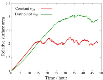
Fig. 10 shows the relative surface areas over time. The relative surface area Srel was defined as follows,
(7) where Ssurf is surface area, and Sini is initial area and
9.0 × 104μm2 in this simulation. The relative surface area by the simulation with distributed vGB was 1.5 times larger compared with that with constant vGB. This result indicates the increase of surface area occurred by remaining grains.
ini rel Ssurf
S = S
Fig. 9. Quarter views of intergranular corrosion simulation; (a) and (b) are same as Fig. 8
Fig. 10. Relative surface area over time
Fig. 11. Cross-sectional view of intergranular corrosion simulation on [100] plane including maximum corrosion depth. (a) and (b) are same as Fig. 8
the results. This indicates that the deepest point of intergranular corrosion tend to be deeper than the value expected from weight loss of specimen, and the difference is roughly 50 μm (average radius of grains) or more.
In this study, we only compared the shapes of intergranular corrosion, and did not compare the corrosion rates.
However, since the simulation could reproduce the shape of intergranular corrosion of experiment could be reproduced very well, we can expect to estimate long- term intergranular corrosion using appropriate vbulk and vGB, which are obtained from initial stage of intergranular corrosion experiments.
5. Conclusions
In this study, three dimensional intergranular corrosion simulation of stainless steel in boiling nitric acid solution was conducted. The results were concluded as follows.
(1) Three dimensional computational model for intergranular corrosion simulation using cellular automata method was developed.
(2) Surface roughness was related to distribution of dissolution rates of grain boundaries and existence of the distribution promote surface roughness.
References
1. K. Osozawa and H. -J. Engell, The anodic polarization curves of iron-nickel-chromium alloys, Corrosion Sci- ence, 6, 389 (1966). Doi: https://doi.org/10.1016/S0010- 938X(66)80022-7
2. F. Ueno, C. Kato, T. Motooka, S. Ichikawa, and M.
Yamamoto, Corrosion Phenomenon of Stainless Steel in Boiling Nitric Acid Solution Using Large-Scale Mock-Up of Reduced Pressurized Evaporator, Journal Nuclear Sci- ence Technology, 45, 1091, (2008). Doi: https://www.tand- fonline.com/doi/abs/10.1080/18811248.2008.9711897 3. J. S. Armijo, Intergranular Corrosion of Nonsensitized
Austenitic Stainless Steels, Corrosion, 24, 24 (1968).
Dependent Intergranular Corrosion Mechanism in Stain- less Steels, Tetsu-to-Hagane, 79, 706 (1993). Doi: https://
doi.org/10.2355/tetsutohagane1955.79.6_706
6. S. Abe, M. Kaneko, H. Komatsu, and F. Kurosawa, The Compound Dependent Intergranular Corrosion Mecha- nism in Stainless Steels, Tetsu-to-Hagane, 79, 713 (1993).
Doi: https://doi.org/10.2355/tetsutohagane1955.79.6_713 7. A. Ohno, H. Isoo, and M. Akashi, Proc. Int. Symp. Plant
Aging Life Prediction of Corrodible Structure, p. 869, Japan Society of Corrosion Engineering, Sapporo, Japan (1995).
8. V. Bague, S. Chachoua, Q. T. Tran, and P. Fauvet, Determination of the long-term intergranular corrosion rate of stainless steel in concentrated nitric acid, Journal of Nuclear Materials, 392, 396 (2009). Doi: https://
doi.org/10.1016/j.jnucmat.2008.12.100
9. T. Igarashi, A. Komatsu, T. Motooka, F. Ueno, Y. Kaji, and M. Yamamoto, Simulations of Intergranular Corro- sion Feature for Stainless Steel using Cellular Automata Method, Zairyo-to-Kankyo, 63, 431 (2014). Doi: https://
doi.org/10.3323/jcorr.63.431
10. H. Gutowitz, Cellular automata?: theory and experi- ment, 1st ed., p. 1, MIT Press (1991).
11. D. Luke, Stellations of the Rhombic Dodecahedron, The Mathematical Gazette, 41, 189 (1957). Doi: https://
doi.org/10.2307/3609190
12. A. I. Adamatzky, Voronoi-like partition of lattice in cellular automata, Mathematical and Computer Modelling, 23, 51 (1996). Doi: https://doi.org/10.1016/0895-7177(96)00003-9 13. A. Komatsu, T. Motooka, M. Makino, K. Nogiwa, F.
Ueno, and M. Yamamoto, Effect of Local Segregation of Phosphorous on Intergranular Corrosion of Type 310 Stainless Steel in Boiling Nitric Acid, Zairyo-to-Kankyo, 63, 98 (2014). Doi: https://doi.org/10.3323/jcorr.63.98 14. R. Courant, K. Friedrichs, and H. Lewy, On the Partial
Difference Equations of Mathematical Physics, IBM Journal of Research Development, 11, 215 (1967). Doi:
https://doi.org/10.1147/rd.112.0215
15. J. Ahrens, B. Geveci, and C. Law, ParaView: An End- User Tool for Large Data Visualization, Visualization
Handbook, p.1, Elsevier (2005).
16. R. Y. Rubinstein and D. P. Kroese, Simulation and the Monte Carlo Method, 2nd ed., p. 1, Wiley-Interscience (2007).
17. J. Nakayama, T. Noura, H. Yamada, and K. Yamamoto, Kobe Steel Engineering Reports, 59, 94 (2009). Doi:
https://www.kobelco.co.jp/technology-review/pdf/59_2/
094-097.pdf
18. I. Ioka, C. Kato, K. Kiuchi, and J. Nakayama, Proc. 16th Int. Conf. Nucl. Eng., p. 48776, American Society of Mechanical Engineering, Orland, Florida, USA (2008).