54: 49 ∼ 60, 2021 April pISSN: 1225-4614 · eISSN: 2288-890X
Published under Creative Commons license CC BY-SA 4.0 http://jkas.kas.org
C OMPARISON OF LOS D OPPLER V ELOCITIES AND N ON - THERMAL L INE
W IDTHS IN THE O FF - LIMB S OLAR C ORONA M EASURED S IMULTANEOUSLY BY C O MP AND H INODE /EIS
Jae-Ok Lee1, Kyoung-Sun Lee2, Jungjoon Seough1, and Kyung-Suk Cho1,3
1Korea Astronomy and Space Science Institute, Daejeon 34055, Korea; [email protected]
2Department of Physics and Astronomy, Seoul National University, Seoul 08826, Korea
3University of Science and Technology, Daejeon 34055, Korea Received February 3, 2021; accepted March 30, 2021
Abstract: Observations of line of sight (LOS) Doppler velocity and non-thermal line width in the off-limb solar corona are often used for investigating the Alfv´en wave signatures in the corona. In this study, we compare LOS Doppler velocities and non-thermal line widths obtained simultaneously from two different instruments, Coronal Multichannel Polarimeter (CoMP) and Hinode/EUV Imaging Spectrometer (EIS), on various off-limb coronal regions: flaring and quiescent active regions, equatorial quiet region, and polar prominence and plume regions observed in 2012–2014. CoMP provides the polarization at the Fe xiii 10747
˚A coronal forbidden lines which allows their spectral line intensity, LOS Doppler velocity, and line width to be measured with a low spectral resolution of 1.2 ˚A in 2-D off limb corona between 1.05 and 1.40 RSun, while Hinode/EIS gives us the EUV spectral information with a high spectral resolution (0.025 ˚A) in a limited field of view raster scan. In order to compare them, we make pseudo raster scan CoMP maps using information of each EIS scan slit time and position. We compare the CoMP and EIS spectroscopic maps by visual inspection, and examine their pixel to pixel correlations and percentages of pixel numbers satisfying the condition that the differences between CoMP and EIS spectroscopic quantities are within the EIS measurement accuracy: ±3 km s−1 for LOS Doppler velocity and ±9 km s−1 for non-thermal width.
The main results are summarized as follows. By comparing CoMP and EIS Doppler velocity distributions, we find that they are consistent with each other overall in the active regions and equatorial quiet region (0.25 ≤ CC ≤ 0.7), while they are partially similar to each other in the overlying loops of prominences and near the bottom of the polar plume (0.02 ≤ CC ≤ 0.18). CoMP Doppler velocities are consistent with the EIS ones within the EIS measurement accuracy in most regions (≥ 87% of pixels) except for the polar region (45% of pixels). We find that CoMP and EIS non-thermal width distributions are similar overall in the active regions (0.06 ≤ CC ≤ 0.61), while they seem to be different in the others (−0.1 ≤ CC
≤ 0.00). CoMP non-thermal widths are similar to EIS ones within the EIS measurement accuracy in a quiescent active region (79% of pixels), while they do not match in the other regions (≤ 61% of pixels);
the CoMP observations tend to underestimate the widths by about 20% to 40% compared to the EIS ones. Our results demonstrate that CoMP observations can provide reliable 2-D LOS Doppler velocity distributions on active regions and might provide their non-thermal width distributions.
Key words: Sun: corona — Sun: infrared — Sun: UV radiation — techniques: spectroscopic — techniques:
imaging spectroscopy — techniques: polarimetric 1. INTRODUCTION
It is generally believed that Alfv´en waves in the solar corona are one of the main energy sources for coro- nal heating and solar wind acceleration. For the last decade, many studies have attempted to find observa- tional evidence for coronal Alfv´en waves by using the Coronal Multi-channel Polarimeter (CoMP, Tomczyk et al. 2008) and/or the Atmospheric Imaging Assem- bly (AIA; Lemen et al. 2012) instrument onboard the Solar Dynamic Observatory (SDO;Pesnell et al. 2012).
CoMP measures the linear polarization of the Fe xiii 10747 and 10798 ˚A coronal forbidden emission lines, and provides their peak intensity, line of sight (LOS)
Corresponding author: J.-O. Lee
Doppler velocity, and line width simultaneously over a field of view (FOV) ranging from 1.05 to 1.40 RSunwith high spatial resolutions of 4.5 arcsec/pixel and temporal cadences of 30 seconds by using three-wavelength data of the Fe xiii lines. For example, three spectral lines (10745, 10746.2, and 10747.4 ˚A) are used for measuring the spectroscopic quantities of the 10747 ˚A coronal line.
By analyzing CoMP LOS Doppler velocity variations along the coronal structures (e.g., coronal loops above active regions and polar plumes), several studies have found outward propagating oscillation patterns in the LOS directions (in other words, transverse directions) to the coronal structures (Tomczyk et al. 2007; Tom- czyk & McIntosh 2009;Threlfall et al. 2013;Liu et al.
2015; Morton et al. 2015, 2016). They interpreted the 49
oscillation patterns as coronal Alfv´en waves because of the following observational characteristics: (1) the oscillations seem to propagate along the coronal struc- tures (magnetic field lines), (2) their phase speeds are much larger than the sound speeds, and (3) there are no oscillation patterns in the intensity, which means that the oscillations are incompressible. Furthermore, by applying the Fourier analysis technique to the LOS Doppler velocity variations, several studies have found the following characteristics: First, the observed waves in the specific frequency ranges near 3 mHz are driven by solar p-modes (Tomczyk et al. 2007; Tomczyk &
McIntosh 2009;Threlfall et al. 2013;Morton et al. 2015, 2016). Second, the waves can be separated into outward- and inward propagating waves (Tomczyk & McIntosh 2009;Threlfall et al. 2013;Morton et al. 2015). Third, the waves might be dissipated by turbulent processes, caused by nonlinear interactions between outward- and inward-propagating waves (Tomczyk & McIntosh 2009;
Moortel et al. 2014;Liu et al. 2014;Morton et al. 2015).
The above findings show that the LOS Doppler velocities by CoMP provide unique observations for examining propagating coronal Alfv´en waves and their origin and dissipation. Several studies showed that the observed oscillation patterns can be interpreted as fast kink waves, not pure torsional Alfv´en waves (Van Doorsselaere et al. 2008; Goossens et al. 2009). Hereafter, we adopt Alfv´enic waves to explain the waves observed by imag- ing instruments such as CoMP and SDO/AIA.
Alfv´en waves can cause non-thermal plasma mo- tions (e.g., transverse motions along the magnetic field lines) which are observed as a broadening of the non- thermal widths of optically thin spectral lines; therefore, the observed non-thermal widths are often used as an indicator of the Alfv´en waves. Several studies attempted to find the observational signatures of Alfv´en waves and their dissipation above the solar limbs with the Extreme Ultraviolet Imaging Spectrometer (EIS;Culhane et al.
(2007)) on board Hinode (Kosugi et al. 2007). Here, the EIS measures high resolution spectra in two wavelength bands, 170–211 ˚A and 246–292 ˚A, with a spectral reso- lution of 0.0223 ˚A/pixel and with different sizes of slits (100and 200) and slots (4000and 26600). EIS provides the spectral line intensities, LOS Doppler velocities, and line widths simultaneously at specific slit positions up to 1.5 RSun. The non-thermal widths can be estimated by removing thermal and instrumental widths from the observed line widths. By analyzing coronal density sen- sitive line pairs of Fe xii 186.88 ˚A and 195.12 ˚A, with the strongest line being that at 195.12 ˚A,Banerjee et al.(2009) have estimated coronal electron densities and non-thermal widths, and examined their relationship in a polar coronal hole observed at the heights between 1.0 and 1.15 RSun. They showed that the non-thermal width is inversely proportional to the square root of the electron density, and this tendency is consistent with the result predicted for undamped radially propagat- ing linear Alfv´en waves. They also showed that the non-thermal width increases with height. Their findings confirmed that non-thermal widths are observational
signatures of Alfv´en waves, and that they are related to the wave amplitudes (Banerjee et al. 1998;Wilhelm et al. 2004). Several studies investigated the observed non-thermal widths in polar coronal holes up to 1.4 RSun
(Bemporad & Abbo 2012;Hahn et al. 2012). They found that the non-thermal widths decrease with increasing height from 1.14 to 1.4 RSun, indicating Alfv´en wave damping in the lower solar corona. This Alfv´en wave damping is also confirmed in active and quiet coronal re- gions (Hahn & Savin 2014;Lee et al. 2014;Gupta 2017;
Zanna et al 2019). These findings show that the non- thermal widths measured with EIS are especially suited to examine coronal Alfv´en waves and their dissipation.
It should be noted that the normal exposure times of EIS for polar coronal hole observations are longer than 100 seconds at a given slit position, and several polar coronal hole studies used EIS data which are binned over more than 20 pixels in the radial direction and/or averaged over observation times of several hours in order to increase the signal-to-noise ratio (Banerjee et al. 2009;
Hahn et al. 2012;Bemporad & Abbo 2012). Therefore, the EIS results usually show structures averaged spa- tially and/or in time. In addition, EIS has a limited field of view with a specific slit location.
As described before, the CoMP provides the in- tensity, LOS Doppler velocity and line width of Fe xiii coronal lines in 2-D for the off limb corona between 1.05 and 1.40 RSun, while it usually obtains three-wavelength data at the Fe xiii lines with a low spectral resolution of 1.2 ˚A. The limitations of the CoMP measurement accuracies are likely to affect the Doppler velocity and non-thermal line width measurements. For example, if the actual spectral line window including strong emis- sion lines is broader than the observed line window (3.6 ˚A), the measured CoMP non-thermal line widths might be underestimated. If the actual spectral window is narrower than the spectral resolution (1.2 ˚A), the measured values might be overestimated. Therefore, in this study, we examine whether the CoMP LOS Doppler velocity and non-thermal width obtained by using only the three-wavelength data are reliable or not. For this, we compare the two physical quantities measured simul- taneously from CoMP Fe xiii 10747 ˚A lines and EIS Fe xii 195.12 ˚A lines for investigating flaring and quies- cent active regions. The EIS Fe xiii 202.04 ˚A lines are used for examining an equatorial quiet region, a polar prominence region, and a polar plume region. Here, about twenty wavelength data sets (spectral lines rang- ing from 194.9 to 195.4 ˚A and from 201.8 to 202.3 ˚A) of the EIS Fe xii and Fe xiii lines, corresponding to a high spectral resolution of 0.025 ˚A are used to derive spectroscopic quantities.
This paper is organized as follows. In Section2, we describe the data and the analyses to determine LOS Doppler velocities and non-thermal widths of CoMP and EIS observations. We also show the comparison method for the spectroscopic quantities. In Section3, we provide results for the various coronal regions observed in 2012–2014 at the heights from 1.05 to 1.25 RSun. A brief summary and discussion are presented in Section4.
2. DATA ANDANALYSIS
2.1. Data
We use the Heliophysics Knowledgebase Event (HEK) search1 to select the EIS observations. The HEK offers solar event lists (e.g., coronal mass ejections or active regions) with available solar data (e.g., SDO/AIA and EIS), and we can make our own event list by using fil- tering keywords (e.g., instruments and locations). For data selection, we use the following procedure: (1) We extract 1003 EIS observations including all measure- ment modes (e.g., slit and slot observations) from 2011 to 2018 by using the HEK search with the following criteria: EIS observations are located between 850 and 1140 (−840 and −1140) in Solar x and y directions to select off-limb observations; (2) we select 180 EIS data sets whose observation times are similar to CoMP ones by using the daily movies of CoMP intensities in the CoMP online database;2 and (3) finally, we use 7 EIS observations which satisfy the following conditions:
First, they are slit observations and include the Fe xii 195.12 ˚A and/or Fe xiii 202.04 ˚A lines. The pixel res- olution of EIS is determined by the observation mode (slit or slot). The EIS observations used in our study used a slit width of 200 with a pixel resolution of 200 in x direction and 100 in y direction. The slit scans the target regions from solar west to east to produce a raster image. Depending on the observing program, the scan- ning steps along the x direction are different. Second, during the times of EIS observations, coronal structures and their spectroscopic quantities are clearly identified in the CoMP Fe xiii 10747 ˚A observations. The seven EIS observations and the related CoMP observations are summarized in Table 1. The EIS center position is recalculated after aligning EIS raster scan images to SDO/AIA 193 ˚A images at the mid-time of each raster scan. The EIS and CoMP data are taken from the EIS online database3 and the CoMP online database. The SDO/AIA data are provided by the Korean Data Center (KDC) for SDO.4
2.2. Determination of LOS Doppler Velocity and Non-thermal Width
For the CoMP observations, we use level 2 dynamic data obtained from three-point spectral line observations of Fe xiii 10747 ˚A following the data reduction process described by Tomczyk et al.(2008) and the calculation process given byTian et al.(2013). The dynamic data directly provide peak intensity, LOS Doppler velocity, and line width images. In order to construct a map of non-thermal line widths, we subtract the thermal width (21 km s−1, corresponding to the peak formation tem- perature of Fe xiii of ∼1.6 MK) and instrumental width (21 km s−1) calculated byMorton et al.(2015) from the line width obtained for each pixel. Since the CoMP
1https://www.lmsal.com/heksearch
2https://mlso.hao.ucar.edu/mlso_data_calendar.php?
calinst=comp
3http://solarb.mssl.ucl.ac.uk/SolarB/SearchArchive.jsp
4http://sdo.kasi.re.kr
Doppler velocities in the faint coronal structures have large measurement errors, described in the CoMP L2 Data Guide document,5we only consider CoMP spectro- scopic data where the CoMP intensities are higher than 20% of the maximum intensities. It should be noted that the CoMP LOS Doppler velocity is partially corrected for the solar rotation effect (blueshift dominates at the east limb while redshift prevails at the west limb) through a method developed byTian et al. (2013) who use the median value of the LOS Doppler shift in each map as the zero point for estimating the LOS Doppler velocity.
Therefore, the CoMP LOS Doppler velocities are relative velocities rather than absolute ones. The dynamic data directly provide peak intensity, LOS Doppler velocity, and line width images calculated analytically from the intensities observed at three wavelength points within the CoMP spectral window (Tian et al. 2013;Morton et al. 2016). The measurement uncertainties for the CoMP Doppler velocities are determined from the intensity measurement errors by error propagation. Morton et al.
(2016) compared analytic uncertainties on the Doppler velocity measurements to the root mean square values of noise calculated from the data. The result showed that the root mean square errors of intensity noise are comparable to the uncertainty of the Doppler velocity measurement. Therefore, the faint structures having low signal to noise have large Doppler velocity measurement errors, which is described in the CoMP L2 data guide document. For the measurement errors on line widths, there are no reports to the best of our knowledge. How- ever, the uncertainties of the line width measurements are also determined by the intensity errors. Therefore, we only consider those CoMP spectroscopic data where the intensities are higher than 20% of the maximum intensities.
For the EIS observations, we follow the standard procedure of EIS data analysis in the Solar Software.
We use the routine eis prep.pro to convert EIS level 0.0 data into level 1.0 data, which are corrected for the CCD dark current, warm pixel, and cosmic ray effects.
We then select the spectral line range 194.9–195.4 ˚A (201.8–202.3 ˚A) for the analysis of Fe xii 195.12 ˚A (Fe xiii 202.04 ˚A). In order to increase the signal-to- noise ratio of EIS data for weak lines and to match their spatial resolution (1 arcsec/pixel in y direction) to that of CoMP (4.35 arcsec/pixel), we apply four-pixel binning in y direction to EIS data using the routine eis bin windata.pro. All EIS spectral line profiles are fitted with a single Gaussian function by using the routine eis auto fit.pro. We correct for the periodic variation of the center position of the EIS spectral line caused by the orbital motion of the Hinode spacecraft using the routine eis update fitdata.pro. Finally, we obtain the intensity, Doppler velocity, and non-thermal width maps and their measurement error maps for each EIS observation using eis get fitdata.pro. When subtracting the thermal width, we assume that the peak formation temperatures of Fe xii and Fe xiii are 1.6
5https://mlso.hao.ucar.edu/CoMPL2DataGuide.pdf
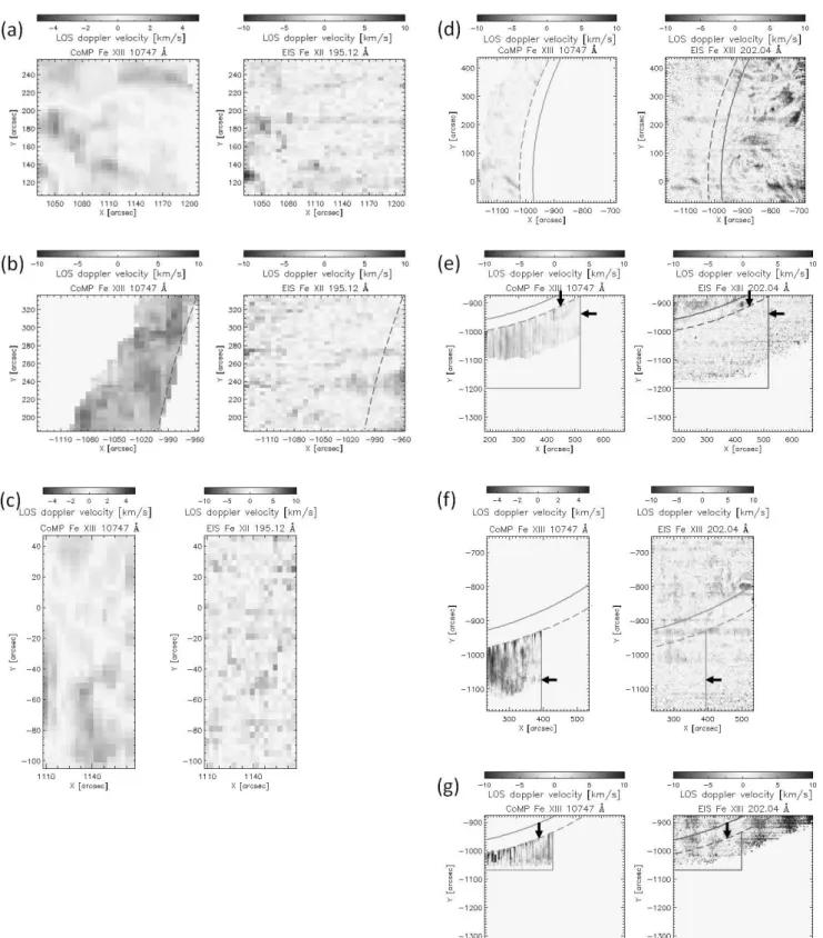
Figure 1. Raster scan CoMP and EIS intensity maps for all coronal regions. The panels show the flaring active region (a), quiescent active regions (b and c), equatorial quiet region (d), polar prominence regions (e and f), and polar plume region (g).
These are corresponding to event Nos. 1–7 in Table1. In each raster scan map, the y direction shows spatial variations at a given time, while the x direction represents temporal and spatial variations. Green and blue contours show the regions where CoMP intensities are equal to 20% and 50% of their maximum intensities, respectively. In panel (c), all pixels have values higher than 20% of the maximum intensities. The gray continuous (dashed) partial circle lines indicate the solar disk (CoMP occulting disk). In panels (e–g), the yellow and yellow-dotted arrows indicate the observed prominence and polar plume, respectively. The horizontal and vertical gray lines represent the observed CoMP FOV in its pseudo raster scan. Limitations of the CoMP FOVs in solar x direction are caused by CoMP data gaps during the EIS raster scan observations as shown in columns 4 and 12 of Table 1. The data gaps are caused by limitations on the available time windows due to geographic and weather conditions of the ground-based CoMP observations.
Figure 2. Raster scan CoMP and EIS Doppler maps. Each panel shows the same events as in Figure 1. We only present CoMP Doppler velocities for locations where the CoMP intensity is higher than 20% of the maximum intensity, and EIS velocities where the EIS measurement error is below the measurement accuracy (±3 km s−1). In panels (e–g), black arrows indicate specific regions where the LOS Doppler velocity patterns are similar in both CoMP and EIS observations. The gray partial circle (dashed circle) and horizontal (vertical) gray lines are the same as those in Figure1.
and 2.0 MK, respectively, according to the CHIANTI database version 7.0. The instrumental widths are pro- vided by the EIS software note 7 (Young 2011). Since the EIS measurement accuracies for LOS Doppler veloc- ities and line widths are about 3 km s−1 and 9 km s−1, respectively, according to the EIS online database,6 we only consider EIS spectroscopic data with measurement errors within the measurement accuracies. It should be noted that there are no absolute reference wave- lengths for estimating the EIS LOS Doppler velocity.
Therefore, the LOS Doppler velocity depends on the reference wavelength and is relative velocity. In the routine eis auto fit.pro the reference wavelength is automatically set to be the average centroid of the line over the raster scan. The reference wavelengths are given in Table1.
2.3. Comparison of CoMP and EIS Observations In order to compare the spectroscopic quantities ob- tained from CoMP and EIS data, we construct pseudo raster scan CoMP maps (e.g., intensity, LOS Doppler velocity, and non-thermal width maps) by using the time and slit position for each EIS scan. Since CoMP and EIS data have slightly different temporal cadences and spatial resolutions, we use the following procedure:
First, we select the closest CoMP images before or after EIS raster scans under the condition that time differ- ences between CoMP observations and EIS raster scans should be smaller than 30 seconds. Second, we take the pixels closest to the scan positions. By using the CoMP and EIS raster scan intensity maps, we check the co-alignment of CoMP and EIS data. Figure 1shows the CoMP and EIS intensity maps for all events. We find that they are spatially and temporally consistent overall. When we examine their pixel-to-pixel correla- tions, the correlation coefficients (CCs) are generally high, ranging from 0.70 to 0.98 (average of 0.91 and median of 0.95). After confirming the co-alignment, we compare the CoMP and EIS LOS Doppler velocity (non-thermal width) maps by visual inspection, and ex- amine pixel-to-pixel correlations and percentages of pixel numbers satisfying the condition that the differences be- tween CoMP and EIS spectroscopic quantities are within the EIS measurement accuracies. As described before, CoMP and EIS Doppler velocities are relative velocities.
Therefore, systematic differences between them might exist. We estimate the systematic differences from the peak values of the histograms of the differences between CoMP and EIS Doppler velocities. The differences are corrected for estimating the percentages of pixels mea- sured to within the EIS measurement accuracy. In order to check whether or not the statistical results between CoMP and EIS spectroscopic quantities depends on the coronal brightness, we apply the same analysis to two sub-coronal regions: relatively bright structures whose CoMP intensities are higher than 50% of their maximum intensities and faint structures whose CoMP intensities
6https://hinode.nao.ac.jp/en/for-researchers/
instruments/eis/fact-sheet
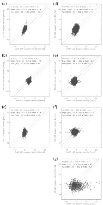
Figure 3. CoMP vs. EIS LOS Doppler velocities. Each panel shows the same event as the corresponding panel of Figure1.
The dashed lines indicate equality of the two spectroscopic quantities, while the upper and lower dotted lines indicate the EIS measurement accuracy for determining Doppler veloci- ties (±3 km s−1). Since the systematic differences between CoMP and EIS Doppler velocity observations are estimated as 4, −2, −2, and −2 km s−1 shown in Figure4b, e, f, and g, respectively, we shift the equality and EIS measurement accuracy lines in panels b, e, f, and g accordingly. CC and RMSE indicate correlation coefficient and root mean square error, respectively. The red and blue symbols indicate rela- tively bright and faint structures as described in Section2.2.
The Doppler velocities of bright structures overlap with those of faint structures.
are higher than 20% and less than or equal to 50% of the maximum intensities.
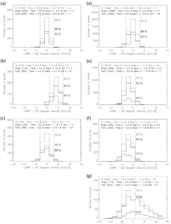
Figure 4. Histograms of the differences between CoMP and EIS LOS Doppler velocities with a bin size of 2 km s−1. The pixel numbers within vertical lines indicate that the differ- ence between CoMP and EIS Doppler velocities are within the EIS measurement accuracy. The systematic differences between CoMP and EIS Doppler velocity observations are estimated as 4, −2, −2, and −2 km s−1in panels b, e, f, and g, respectively. These are corrected for estimating the per- centages of pixels measured to within the EIS measurement accuracy. The percentages are presented in each histogram.
“Std” indicates standard deviation. The red and blue symbols are the same as those in Figure2.
3. RESULTS
3.1. Relationships between CoMP and EIS LOS Doppler Velocities
Figure 2shows CoMP and EIS LOS Doppler velocity maps. By comparing the LOS Doppler velocity maps for all coronal regions, we find that they are spatially and temporally consistent overall in the active regions and equatorial quiet region (Figures 2a–d), while they are partially similar to each other in the overlying loops of prominences (black arrows in Figures2e–f) and near the bottom of the polar plume (Figure 2g). We quantita- tively investigate relationships between CoMP and EIS LOS Doppler velocity distributions and their difference histograms as shown in Figures 3 and4. CoMP and EIS Doppler velocity distributions show higher corre- lation coefficients (CC) in the active regions and the equatorial quiet region (0.25 ≤ CC ≤ 0.7) than in the other coronal regions (0.02 ≤ CC ≤ 0.18) as shown in
Figure 3. For the flaring active region with the high- est correlation coefficient (CC = 0.7), the slope of the linear regression is about 1.23. The Doppler velocities measured from EIS are larger than the CoMP ones by a factor of 1.2. Figure4shows the percentages of pixels for which the difference of the Doppler velocities mea- sured from the two different instruments is within the EIS measurement accuracy (±3 km s−1). The velocity differences are within the EIS measurement accuracy in most coronal regions (≥87% of pixels) except for the polar plume region (45% of pixels) when considering the systematic differences due to the determination of the reference wavelength. Our results demonstrate that CoMP observations that only provide three-wavelength photometry around the Fe xiii forbidden lines can pro- vide reliable 2-D LOS Doppler velocity distributions on active regions and the equatorial quiet region.
When examining two sub-coronal regions selected according to their CoMP intensities (relatively bright structures whose CoMP intensities are higher than 50%
of the maximum intensities and faint structures whose CoMP intensities are 20–50 % of the maximum inten- sities), we find the following statistical characteristics:
First, the bright structures in the relatively bright coro- nal regions (active regions and equatorial quiet region) show slightly stronger correlations (0.28 ≤ CC ≤ 0.79) than the faint structures (0.12 ≤ CC ≤ 0.59), while there seems to be no difference in faint coronal regions (polar prominence and plume regions). Second, the CoMP Doppler velocity distributions are consistent with the EIS ones within the EIS measurement accuracy in most regions (≥76% of pixels for bright structures and ≥89%
of pixels for faint structures) except for the polar region (47% for bright structures and 44% for faint structures).
In addition to that, the slopes of the linear regressions are about 1.47 and 1.58 for the bright structures in the flaring and quiescent active regions (event Nos. 1 and 2, respectively) with higher correlation coefficients (CC ≥ 0.72). This implies that the EIS Doppler velocities are larger than the CoMP ones by a factor of 1.5 in bright structures in active regions.
3.2. Relationships between CoMP and EIS LOS Non-thermal Line Widths
Figure 5shows CoMP and EIS LOS non-thermal line width maps. By analyzing the non-thermal width maps for all coronal regions, we find that they seem to be similar overall in the active regions (Figure5a–c) while showing different observational tendencies: the relatively bright structures near the solar limb have higher (lower) non-thermal widths than the faint ones far from the solar limb in flaring active region as shown in Figure5a (quiescent active regions as shown in Figure5b–c). In the equatorial quiet and polar prominence regions shown in Figure 5d–f, they are different from each other: the EIS non-thermal widths are higher in relatively bright structures, while there seem to be no systematic differ- ences for the CoMP non-thermal widths. Since the EIS observations provide limited non-thermal width maps in the polar plume region (Figure5g), we cannot compare
Figure 5. Raster scan CoMP and EIS non-thermal width maps. We only present CoMP non-thermal widths where CoMP intensities are higher than 20% of the maximum intensity, and EIS non-thermal widths where its measurement error is within the measurement accuracy (±9 km s−1) and its line width is larger than the sum of thermal and instrumental widths. The gray partial circle (dashed circle) and horizontal (vertical) gray lines are the same as those in Figure1.
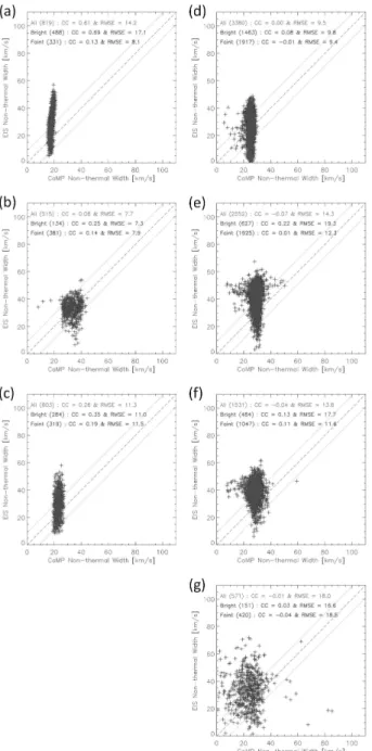
Figure 6. CoMP vs. EIS non-thermal widths. Each panel shows the same events as in Figure 1. The dashed lines indicate equality of the two spectroscopic quantities, while the upper and lower dotted lines indicate the EIS measure- ment accuracy for determining line widths (±9 km s−1). The non-thermal widths of bright structures overlap with those of faint structures. CC, RMSE, red symbols, and blue symbols are the same as in Figure3.
them. We quantitatively examine relationships between CoMP and EIS LOS non-thermal width distributions and their difference histograms shown in Figures6 and 7. They show overall positive correlations in the active regions (0.06 ≤ CC ≤ 0.61) and marginal negative cor- relations in the others (−0.1 ≤ CC ≤ 0.0) as shown in Figure 6. For the flaring active region with the highest correlation coefficient (CC = 0.61) the slope of the linear
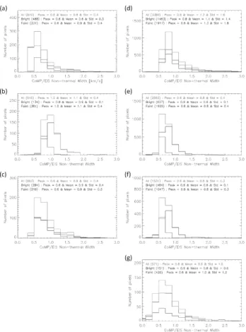
Figure 7. Histograms of the differences between CoMP and EIS LOS non-thermal widths with a bin size of 6 km s−1. Each panel shows the same events in Figure 1. The pixel numbers within vertical lines indicate that the difference between CoMP and EIS non-thermal widths are within the EIS measurement accuracy. The red and blue symbols are the same as in Figure3. The percentages and Std are the same as those in Figure4.
regression is about 5.7, indicating that EIS non-thermal widths are about six times larger than CoMP ones. This trend is caused by the limited non-thermal width range (15.2–21.2 km s−1) in CoMP observations compared to the EIS ones (5.1—57.1 km s−1). The percentages of pixels with line widths within the EIS measurement accuracy (±9 km s−1) are ≤61% in most regions except for the quiescent active region (AR 12149) in 2012 April 16 as shown in Figure5b (79%). When examining the ratio histograms for the CoMP and EIS non-thermal widths shown in Figure8, we find that the peak values range from 0.6 to 0.8, indicating that CoMP underesti- mates the line widths by about 20% to 40%. Our results indicate that even though the CoMP non-thermal line widths tend to be too low by about 30%, the CoMP data can provide non-thermal width distributions in active regions.
When examining the CoMP intensities in two sub- coronal regions, we find the following statistical trends:
First, bright structures have somewhat higher correla- tions (0.03 ≤ CC ≤ 0.69) than faint structures (−0.04 ≤ CC ≤ 0.19) on all coronal regions. Second, the percent-
Figure 8. Histograms of the ratios of CoMP and EIS LOS non-thermal widths with a bin size of 0.2. Each panel shows the same events as in Figure1. The red and blue symbols are the same as in Figure3. Std is the same as in Figure4.
ages of pixels with intensities within the EIS measure- ment accuracy are lower in bright structures (2–75%) than in faint structures (45–80%) in most regions ex- cept for the active region AR 12149 (bright structures:
57%, faint structures: 56%) and the polar plume region (bright structures: 44%, faint structures: 39%). The CoMP observations tend to underestimate the inten- sities more, by about 37%, in bright structures than in faint structures (by about 30%) in most coronal re- gions except for AR 12149 (bright structure: 20%, faint structure: 0%). In addition to that, we note that the slope of the linear regression is about 5.7 for the bright structures in the flaring active region with the highest correlation coefficient (CC = 0.69). This implies that the EIS non-thermal widths are much larger than the CoMP ones, by a factor of 6, in bright structures in the flaring active region.
4. SUMMARY ANDDISCUSSION
Over the last decade, the LOS Doppler velocities by CoMP and the non-thermal widths by Hinode/EIS have been used to find observational evidence for coro- nal Alfv´en waves and their origin, dissipation, and en- ergy fluxes. The CoMP provides 2-D information on the intensity, LOS Doppler velocity, and line width of Fe xiii 10747 ˚A coronal forbidden lines for the off-limb
corona between 1.05 and 1.40 RSun, usually using three- wavelength photometric data (at 10745.0, 10746.2, and 10747.4 ˚A) nearby the Fe xiii lines with a low spectral resolution of 1.2 ˚A. In this study, we examine whether the CoMP LOS Doppler velocity and non-thermal width obtained by using only the three-wavelength data are reliable or not. For this, we compare the spectroscopic physical quantities obtained from CoMP Fe xiii 10747 ˚A lines with that from EIS Fe xii 195.12 ˚A or Fe xiii 202 ˚A (spectral windows ranging from 194.9 to 195.4 and from 201.8 to 202.3 ˚A) with a high spectral resolution of 0.025 ˚A. In order to compare them, we make pseudo raster scan CoMP maps using information for EIS scan slit times and positions. We then compare the CoMP and EIS spectroscopic maps by visual inspection, and examine pixel-to-pixel correlations and percentages of pixel numbers satisfying the condition that the differ- ences between CoMP and EIS spectroscopic quantities are within EIS measurement accuracy: ±3 km s−1 for LOS Doppler velocities and ±9 km s−1 for non-thermal widths.
By examining seven data sets from five different coronal regions (flaring and quiescent active regions, equatorial quiet region, and polar prominence and plume regions), we find the following statistical characteristics:
The CoMP and EIS Doppler velocity distributions are consistent overall in the active regions and equatorial quiet region (0.25 ≤ CC ≤ 0.7), while they are simi- lar in the overlying loops of prominences and near the bottom of the polar plume (0.02 ≤ CC ≤ 0.18). The differences of the Doppler velocities are within the EIS measurement accuracy in most coronal regions (≥ 87%
of all pixels) except for the polar plume region (45%
of pixels). These results show that CoMP observations with three-wavelength data provide reliable 2-D LOS Doppler velocity distributions in active regions and equa- torial quiet region. The linear regression for the flaring active region having the highest correlation (CC = 0.7) finds a slope of 1.23, indicating that the EIS Doppler velocities are slightly larger than the CoMP ones by a factor of 1.2. When we only consider relatively bright structures whose CoMP intensities are higher than 50%
of the maximum intensities, the slope is 1.5. These re- sults, together with previous studies of the wave energy flux of propagating Alfv´enic wave signatures by using CoMP Doppler velocity observations (Tomczyk et al.
2007;Threlfall et al. 2013), might suggest that the wave energy flux is about 44% or 125% larger than the one obtained without the corrections found from comparison to EIS observations.
We find that CoMP and EIS non-thermal width dis- tributions are similar overall in the active regions (0.06
≤ CC ≤ 0.61), while they seem to be different in the others (−0.1 ≤ CC ≤ 0.00). CoMP non-thermal widths are similar to EIS ones within the EIS measurement accuracy in a quiescent active region (79% of pixels), while they do not match in the others (≤61% of pixels).
The CoMP line widths are 20–40% smaller than the EIS widths. Our results indicate that although CoMP obser- vations tend to underestimate line widths by about 30%,
Table 1
EIS and CoMP observations.
EIS CoMP
# Coronal regions Date Time Slit center FOV Exp. time Scan step Spec. line Ref. line Data file Time
[yyyy/mm/dd] [UT] (x,y) [00] [00] [sec] [00] [˚A] [sec] [UT]
1 Flaring active region (AR 11654)a 2013/01/20 19:11∼19:16 1120, 181 180×152 11 6 Fe xii 195.1179 eis l0 20130120 191108 19:11∼19:16 2 Quiescent active region (AR 11461) 2012/04/16 22:53∼22:58 -1046, 260 180×152 11 6 Fe xii 195.1149 eis l0 20120416 225303 22:52∼22:59 3 Quiescent active region (AR 12149) 2014/09/01 18:28∼18:32 1138, 29 60×150 11 3 Fe xii 195.1167 eis l0 20140901 182849 18:28∼18:33 4 Equatorial quiet region 2013/02/26 19:07∼20:13 -925, 181 491×512 32 4 Fe xiii 202.0677 eis l0 20130226 190744 19:17∼20:13 5 Polar prominence region 2013/02/25 21:44∼22:50 427, -1129 491×512 32 4 Fe xiii 202.0124 eis l0 20130225 214444 22:05∼22:50 6 Polar prominence region 2013/05/05 18:20∼19:25 373, -920 300×512 52 4 Fe xiii 202.0512 eis l0 20130505 182040 18:50∼19:25 7 Polar plume region 2013/01/17 22:10∼23:16 435, -1133 491×512 32 4 Fe xiii 202.0309 eis l0 20130117 221044 22:44∼23:17
aB7.0 and B4.5 flares continuously occur at 17:05 and 19:17 UT, respectively.
All EIS observations use the 200slit in Solar x direction with different scanning steps (300, 400, and 600). The pixel resolution in Solar y direction is 100. Since there are no observations of Fe xiii 202.04 ˚A in the solar active regions, we use Fe xii 195.12 ˚A. The spatial resolutions and temporal cadences of CoMP observations are about 4.35 arcsec/pixel and 30 seconds, respectively.
they might provide non-thermal width distributions in active regions. When examining the linear regression for the flaring active region having the highest correlation (CC = 0.61), the slope is 5.7, indicating that the EIS non-thermal widths are six times larger than the CoMP ones. This trend is caused by the limited non-thermal width range (15.2–21.2 km s−1) in CoMP observations compared to the EIS ones (5.1–57.1 km s−1). The dif- ferences in non-thermal widths between CoMP and EIS and the limited CoMP non-thermal width range are mainly caused by the limited spectral window (3.6 ˚A) for CoMP observations that use the three-wavelength filters. If we use the five-wavelength filter CoMP obser- vations of Fe xiii 10747 ˚A with a wide spectral window of 10 ˚A as shown in Figure 5 ofTomczyk et al. (2008), the differences might be reduced and the limited non- thermal width range might be broader. We cannot rule out the possibility that using the EIS Fe xiii 202.04 ˚A line instead of Fe xii 195.12 ˚A for comparing non-thermal widths in active regions reduces the differences; the ther- mal width of Fe xiii is about 11% larger than that of Fe xii, which reduces the observed non-thermal widths in EIS observations. For example, comparing the aver- age of non-thermal widths between Fe xii and Fe xiii for four events (Event Nos. 4–7 in Table 1), we find that the non-thermal widths of Fe xiii are about 11% in average (with a range of 2–21%) smaller than those of Fe xii.
From investigating the non-thermal width maps for active regions, we find that the CoMP and EIS non- thermal width distributions are similar overall while showing different trends: CoMP and EIS non-thermal widths of bright structures near the solar limb are larger than those in the faint structures far from the solar limb in the flaring active region, and they are smaller than those in the faint structures in the quiescent active re- gions. The non-thermal width distribution in the flaring active region might be related to Alfv´en wave damping under the assumption that non-thermal plasma motions are mainly caused by the Alfv´en waves. We cannot rule out the possibility that Gaussian fitting errors that occur when determining line widths on maps with small intensity-to-background ratio lead to significant changes in computed non-thermal widths as shown in Figure 10 of Brooks & Warren(2016). The non-thermal width
distributions in quiescent active regions might be con- nected to propagating coronal Alfv´en waves (Banerjee et al. 1998;Wilhelm et al. 2004;Banerjee et al. 2009) or caused by the Gaussian behavior of fits of line widths in low-intensity regions which results in larger full width at half maximum values than in high-intensity regions for given spectral lines.
Our results demonstrate that CoMP observations can provide reliable 2-D LOS Doppler velocity distri- butions in active regions and might provide their non- thermal width distributions. By comparing electron densities on coronal loops within a complex of active regions (AR 12579, 12582, and 12583) obtained from CoMP and Hinode/EIS data,Dud´ık et al.(2021) showed that CoMP observations can provide trustworthy 2-D electron density distributions in active regions. There- fore, CoMP with SDO/AIA observations can be used to detect propagating Alfv´enic (or Alfv´en) wave signatures on different active regions at the same time, and estimate their origins, dissipation, and energy fluxes. According to the theoretical description of Alfv´en-wave turbulence heating (Chandran & Hollweg 2009; Chandran et al.
2011), the efficiency of turbulent heating depends not only on the observed non-thermal width but also on the plasma environment such as the local Alfv´en speed and the plasma β, which is the ratio of plasma pressure to magnetic pressure. Thus, remote-sensing observations might be useful when investigating the turbulent heat- ing rates for different coronal regions, and furthermore, give a better understanding of coronal heating and solar wind acceleration by Alfv´enic (or Alfv´en) waves.
ACKNOWLEDGMENTS
We are grateful to the referees, the scientific editor, and the editor-in-chief for helpful and constructive com- ments. This study was supported by the Korea As- tronomy and Space Science Institute under the R&D program “Development of a Solar Coronagraph on In- ternational Space Station (Project No. 2021-1-850-09)”
supervised by the Ministry of Science, ICT and Fu- ture Planning. This research was also supported by the Basic Science Research Program through the Na- tional Research Foundation of Korea(NRF) funded by the Ministry of Education (2019R1F1A1055071). The work of KSL was supported by NRF grants funded
by the Korean government (NRF-2020R1A2C2004616 and 2021R1A2C1010881). The CoMP data is cour- tesy of the Mauna Loa Solar Observatory, operated by the High Altitude Observatory, as part of the National Center for Atmospheric Research (NCAR). N.C.A.R. is supported by the National Science Foundation. Hin- ode is a Japanese mission developed and launched by ISAS/JAXA, with NAOJ as domestic partner and NASA and STFC (UK) as international partners. It is oper- ated by these agencies in cooperation with ESA and the NSC (Norway). The SDO is the first mission of NASA’s Living With a Star (LWS) Program. SDO data a courtesy of NASA/SDO and the AIA science team.
The SDO data were provided by the Korea Data Center (KDC) for SDO in cooperation with NASA, which is supported by the “Development of Korea Space Weather Research Center” project of the Korea Astronomy and Space Science Institute (KASI). CoMP 1079 nm data DOI:10.5065/D6MG7MJM
REFERENCES
Banerjee, D., Perez-Suarez, D., & Doyle, J. G., 2009, Signa- tures of Alfv´en Waves in the Polar Coronal Holes as Seen by EIS/Hinode, A&A, 501, L15.
Banerjee, D., Teriaca, L., Doyle, J. G., et al. 1998, Broaden- ing of Si viii Lines Observed in the Solar Polar Coronal Holes, A&A, 339, 208.
Bemporad, A., & Abbo, L. 2012, Spectroscopic Signature of Alfv´en Waves Damping in a Polar Coronal Hole up to 0.4 Solar Radii, ApJ, 751, 110.
Brooks, D. H., & Warren, H. P. 2016, Measurements of Non- Thermal Line Widths in Solar Active Regions, ApJ, 820, 63.
Chandran, B. D. G., & Hollweg, J. V., 2009, Alfv´en Wave Reflection and Turbulent Heating in the Solar Wind from 1 Solar Radius to 1 AU: An Analytical Treatment, ApJ, 707, 1659.
Chandran, B. D. G., Dennis, T. J., Quataert, E., & Bale, S. D., 2011, Incorpoating Kinetic Physics into a Two- Fluid Solar-Wind Model with Temperature Anisotropy and Low-Frequency Alfv´en-Wave Turbulence, ApJ, 743, 197.
Culhane, J. L., Harra, L. K., James, A. M., et al. 2007, The EUV Imaging Spectrometer for Hinode, Sol. Phys., 243, 19.
Dud´ık, J., Zanna, G. D., Ryb´ak, J., et al. 2021, Electron Densities in the Solar Corona Measured Simultaneously in the Extreme Ultraviolet and Infrared, ApJ, 906, 118.
Goossense, M., Terradas, J., Andries, J., et al. 2009, On the Nature of Kink MHD Waves in Magnetic Flux Tubes, A&A, 503, 213.
Gupta, G. R. 2017, Spectroscopic Evidence of Alfv´en Wave Damping in the Off-limb Solar Corona, ApJ, 836, 4.
Hahn M., Landi, E., & Savin, D. W., 2012, Evidence of Wave Damping at Low Heights in a Polar Coronal Hole, ApJ, 753, 36
Hahn, M., & Savin, D. W. 2014, Evidence for Wave Heating of the Quiet-Sun Corona, ApJ, 795, 111.
Kosugi, T., Matsuzaki, K., Sakao, T., etal. 2007, The Hinode (Solar-B) Mission: An Overview, Sol. Phys., 243, 3.
Lee, K. -S., Imada, S., Moon, Y.-J., et al., 2014, Spectro- scopic Study of a Dark Lane and a Cool Loop in a Solar Limb Active Region by Hinode/EIS, ApJ, 780, 177.
Lemen, J. R., Title, A. M., Akin, D. J., et al. 2012, The Atmospheric Imaging Assembly (AIA) on the Solar Dy- namics Observatory (SDO), Sol. Phys., 275, 17.
Liu, J., Mcintosh, S. W., Moortel, I. D., et al. 2014, Statistical Evidence for the Existence of Alfv´enic Turbulence in Solar Coronal Loops , ApJ, 797, 7.
Liu, J., Mcintosh, S. W., Moortel, I. D., et al. 2015, On the Parallel and Perpendicular Propagating Motions Visible in Polar Plumes: an Incubator for (Fast) Solar Wind Acceleration?, ApJ, 806, 273
McIntosh, S. W., de Pontieu, B., Carlsson, M., et al. 2011, Alfv´enic Waves with Sufficient Energy to Power the Quiet Solar Corona and Fast solar wind, Nature, 475, 477.
Moortel, I.D., Mcintosh, S. W., Threlfall, J. et al. 2014, Potential Evidence for the Onset of Alfv´enic Turbulence in Trans-Equatorial Coronal Loops, ApJL, 782, L34.
Morton, R.J., Tomczyk, S., & Pinto, R. 2015, Investigating Alfv´enic Wave Propagation in Coronal Open-Field Regions, Nat. Commun., 6, 7813.
Morton, R. J., Tomczyk, S., & Pinto, R. F. 2016, A Global View of Velocity Flutuations in the Corona Below 1.3 Rsun
with CoMP, ApJ, 828, 89.
Olsen, S. I. 1993, Estimation of Noise in Images: An Evalua- tion, CVGIP Graphical Models Image Process., 55, 319 Pesnell, W. D., Thompson, B. J., & Chamberlin, P. C. 2012,
The Solar Dynamics Observatory (SDO), Sol. Phys., 275, 3
Threlfall, J., Moortel, I. D., McIntosh, S. W. et al. 2013, First Comparison of Wave Observations from CoMP and AIA/SDO, A&A, 556, A124.
Tian, H., Tomczyk, S., Mcintosh, S. W., et al., 2013, Ob- servations of Coronal Mass Ejections with the Coronal Multichannel Polarimeter, Sol. Phys., 288, 637.
Tomczyk, S., Card, G. L., Darnell, T., et al. 2008, An In- strument to Measure Coronal Emission Line Polarization, Sol. Phys., 247, 411.
Tomczyk, S., McIntosh, S. W., Keil, S. L., et al. 2007, Alfv´en Waves in the Solar Corona, Science, 317, 1192.
Tomczyk, S. & McIntosh, S. W. 2009, Time-Distance Seis- mology of the Solar Corona with CoMP, ApJ, 697, 1384.
Van Doorsselaere, T., Nakariakov, V. M., & Verwichte, E.
2008, Detection of Waves in the Solar Corona: Kink or Alfv´en?, ApJ, 676, L73.
Wilhelm, K., Dwivedi, B. N., & Teriaca, L., 2004, On the Widths of the Mg x Lines near 60 nm in the Corona, A&A, 415, 1133.
Young, P. 2011, EIS Software Note No. 7
Zanna, G. D., Gupta, G. R., & Mason, H. E. 2019, Exploring the Damping of Alfv´en Waves along a Long Off-Limb Coronal Loop, up to 1.4 Rsun, A&A, 631, A163.