1. 서 론
뇌 소혈관 질환(Cerebral small vessel disease, CSVD)은 노년 계층에게서 매우 흔히 나타나는 신경 계 질환의 일종으로 서서히 뇌혈관의 조직을 손상시 킴으로써 뇌졸중, 치매 그리고 인지 저하 등 노화로 인해 발생되는 질환의 주요 원인으로 작용하고 있다 [1-2]. 하지만, 이처럼 빈번하게 발생하는 주요 질병 이지만 정작 이 질병에 대해 알려진 정보는 그리 많 지 않다. 그 이유는 CT(Computerized Tomography) 나 MRI(Magnetic Resonance Imaging)를 이용하여
얻은 저해상도의 뇌 이미지 정보만으로는 생체 내에 있는 작은 혈관에 대한 정확한 분석을 하기 매우 어 렵기 때문이다[3-5]. 윤호성 등의 연구[27]에서는 뇌 를 분석하기 위해 사용된 MR 영상의 해상도는 256
× 256이고, 단면 이미지의 수는 192장으로 작은 혈관 에 대한 분석을 위한 데이터로는 한계가 있다.
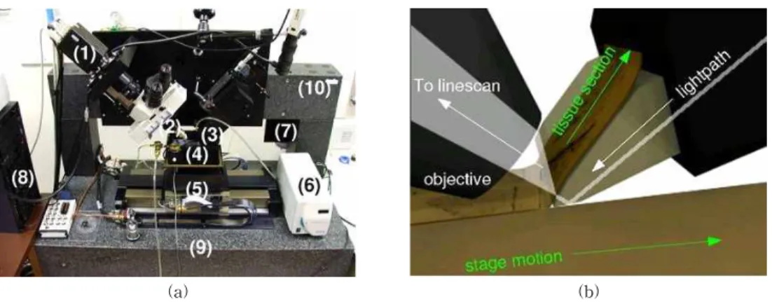
Fig. 1은 Knife-Edge Scanning Microscope(KESM) 로 미국 Texas A&M 대학교의 Brain
Networks 연구실에서 개발된 장비이다[6-7].
KESM을 이용하면 작은 장기(organ)의 단면 이미지 를 0.6 μm × 0.7 μm × 1.0 μm의 복셀(voxel) 해상도
Using Image Threshold Techniques in High-resolution Images of the Mouse Brain
Junseok Lee†
ABSTRACT
In this paper, I lay the foundation for creating a multiscale atlas that characterizes cerebrovasculature structural changes across the entire brain of a mouse in the Knife-Edge Scanning Microscopy dataset.
The geometric reconstruction of the vascular filaments embedded in the volume imaging dataset provides the ability to distinguish cerebral vessels by diameter and other morphological properties across the whole mouse brain. This paper presents a means for studying local variations in the small vascular morphology that have a significant impact on the peripheral nervous system in other cerebral areas, as well as the robust and vulnerable side of the cerebrovasculature system across the large blood vessels. I expect that this foundation will prove invaluable towards data-driven, quantitative investigations into the system-level architectural layout of the cerebrovasculature and surrounding cerebral microstructures.
Key words: Knife-Edge Scanning Microscope, Whole Mouse Brain, Microvascular
※ Corresponding Author : Junseok Lee, Address: (38900) P.O. BOX 135-9, Changha-ri, Gogyeong-Myeon, Yeong- cheon-si, Gyeongsangbuk-do, Korea, TEL : +82-54- 330-4745, FAX : +82-54-335-5790, E-mail : jsleecs@
mnd.go.kr
Receipt date : July 9, 2019, Revision date : Aug. 12, 2019
Approval date : Sep. 2, 2019
†
Dept. of Computer Eng., Korea Army Academy at Yeongcheon
※ This paper is largely based on the author's Ph.D.
Dissertation.
로 이미지를 얻을 수 있으며, 이렇게 추출된 고 해상 도 이미지는 쥐 뇌와 같이 작은 장기의 미세혈관에 대한 정보까지도 포함하게 된다[8]. KESM을 활용하 여 작은 장기의 조직(tissue)을 분석하기 위해 장기 샘플을 준비하고, 샘플의 단면을 자름(cutting)과 동 시에 2D 이미지를 추출하고, 추출된 이미지를 활용 하여 3D 이미지로 복원 및 수학적으로 분석하는 일 련의 과정을 Fig. 2와 같이 시간 순서에 따라 그림으 로 표현하였다.
본 연구에서 사용된 작은 장기는 C57BL/6L 생쥐 의 뇌 이미지를 활용하였으며, 뇌혈관에 대한 분석을 위해 인디아 잉크(India-ink)로 염색된 뇌혈관의 이 미지를 사용하였다[11]. 인디아 잉크로 염색된 뇌혈 관의 이미지는 혈관의 정보도 가지고 있지만, 물리적 으로 장기의 단면을 자르면서 이미지를 추출하는 과 정에서 원하지 않는 노이즈가 포함되기 때문에 다양 한 종류의 이미지 프로세싱 기법이 적용된 사전 작업 을 통해서 노이즈를 제거하는 단계를 거쳐야 한다.
또한, 1 μm 이하의 고해상도로 이미지를 추출하기 때문에 쥐 뇌와 같은 작은 장기의 단면 이 포함된 이미지 데이터 셋의 크기는 대략 1.5 TB 정도로 서브 샘플링(sub-sampling) 단계를 거치지 않으면 이미 지를 다루거나 분석하는데 상당한 시간적 제약과 고 성능의 컴퓨터를 필요로 하게 된다.
본 논문에서는 인디아 잉크로 뇌혈관이 염색된 C57BL/6L 생쥐의 고해상도 뇌 이미지에서 뇌혈관에 대한 정보를 추출하기 위해 이미지 임계화(image threshold) 기법을 활용하여 혈관을 분류하고, 분류 된 이미지 정보를 활용하여 뇌혈관의 지름을 측정하 며 지름의 크기에 따라 뇌혈관 네트워크를 3D로 재 현하고 분석하는 프레임워크(framework)를 제안하 고자 한다. 이 프레임워크는 크게 두 단계로 구성되 어 있다. 첫 번째 부분은 KESM에서 추출된 뇌의 단 면 이미지에서 혈관의 정보만을 얻기 위한 이미지 프로세싱 기법을 언급한다. 두 번째 부분에서는 추출 된 뇌혈관 이미지에서 혈관의 지름 크기에 따라 혈관
(a) (b)
Fig. 1. Knife-Edge Scanning Microscope(KESM). (a) Major components of the KESM are shown: (1) high-speed line- scan camera, (2) microscope objective, (3) diamond knife assembly and light collimator, (4) specimen tank (for water immersion imaging), (5) three-axis precision air-bearing stage, (6) white-light microscope illumina- tor, (7) water pump (in the black) for the removal of sectioned tissue, (8) PC server for stage control and image acquisition, (9) grantie base, and (10) grantie bridge. (b) An illustration of the principle of operation of the KESM. Adapted from [9].
Fig. 2. KESM tissue imaging workflow. It illustrates the process of obtaining a tissue image using KESM. Adapted
from [10].
장에서는 결론을 맺는다.
2. 제안한 방법
2.1 디지털 이미지 프로세싱
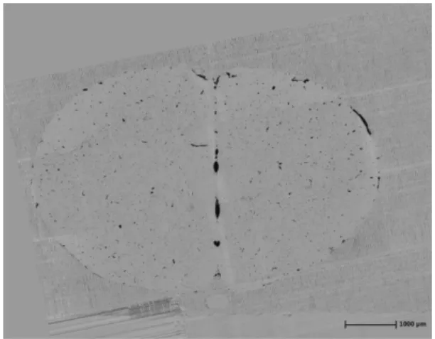
Fig. 3은 KESM에서 추출한 쥐 뇌의 이미지 단면 으로 짙은 검정색 부분은 인디아 잉크로 염색된 뇌혈 관이다. 이 단면 이미지에는 인디아 잉크로 염색된 뇌혈관 정보뿐만 아니라 뇌 영역 외부에 일정한 패턴 을 보이는 노이즈도 역시 존재하고 있으며, 혈관에 대한 정보만을 추출하기 위해서는 다양한 이미지 프 로세싱 기법을 적용하여야 한다. 본 논문에서는 8,560개의 Fig. 3과 같은 뇌의 단면 이미지를 활용하 였으며, 이때 사용된 이미지 해상도는 7,790 px × 6,050 px 이고, 복셀(voxel)의 해상도는 1.2 μm × 1.4 μm × 1.0 μm이다[12].
우선 인디아 잉크로 염색된 혈관의 정보를 추출해 야 하기 위해 쥐 뇌의 이미지 단면을 이진화(binari- zation) 해야 하고, 이를 위해 최소 임계값(minimum
지정하면 그레이 스케일의 이미지를 Fig. 4의 이미지 b와 같이 검은색과 흰색만이 존재하는 이진화 된 이 미지로 만들 수 있다.
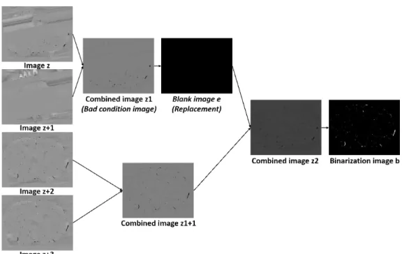
또한, 1.5 TB 크기의 원본 이미지를 분석하기 위해 2단계에 걸쳐 서브샘플링(sub-sampling) 기법을 적 용하였고, 서브샘플링(sub-sampling) 단계에서 손 상된 이미지를 제외하고 연속된 이미지를 결합하는 기법을 추가하여 혈관에 대한 자세한 정보를 얻도록 처리하였다[14]. Fig. 4는 2단계의 서브샘플링(sub- sampling) 과정과 이미지를 이진화 하는 전체 과정 을 표현한 그림이다[14]. 인디아 잉크 데이터 셋을 첫 번째 서브샘플링 하는 과정에서 뇌의 단면 이미지 는 x, y축으로 50% 크기가 작아진다. 이미지의 크기 가 작이진 만큼 z축으로도 단면 이미지의 개수가 50% 줄어야 한다. 최초 8,560개의 단면 이미지에서 우리가 필요로 하는 이미지의 수는 4,280개로 줄어들 게 되며, 이 과정에서 단면 이미지별 보유하고 있는 혈관에 대한 정보를 획득하기 위해 두 이미지를 결합 (픽셀 밝기값의 평균값 적용)하여 한 이미지로 만들 었다. 첫 번째 서브샘플링 과정을 진행하다 보면 Fig.
4의 결합된 이미지 z1과 같이 물리적으로 손상된 이 미지가 만들어 질 수 있다. 이러한 이미지는 두 번째 서브샘플링 과정에서 수동으로 손상된 이미지 z1을 검정색으로 처리된 빈 이미지 e로 교체하는 과정을 통해 손상된 이미지의 정보는 제거되고, 결합된 이미 지 z1+1이 가지고 있는 혈관 정보는 검정색으로 처리 된 빈 이미지 e와 결합하면서 z1+1의 혈관 정보를 그대로 보유하고 있는 이미지 z2가 만들어진다. 손상 되지 않은 이미지는 첫 번째 서브샘플링 과정에서와 같이 두 이미지의 결합이 이루어진다. 결과적으로 본 논문에서는 두 단계의 서브샘플링 기법을 통해 이미 지 데이터 셋의 x, y축은 원본 이미지의 25% 크기가 되며, z축으로는 2,140개의 단면 이미지만을 사용하 게 된다.
Fig. 3. A cross section of the mouse brain. The black
parts are vascular stained with India ink. Coro-
nal view(↑: Dorsan, ↓: Ventral).
2.2 혈관 지름 크기에 따른 분류
이번 장에서는 2.1에서 이미지 프로세싱 결과로 얻은 이진화 된 이미지를 활용하여 뇌혈관의 지름 크기에 따라 혈관 정보를 분류하고 분류된 정보를 바탕으로 혈관 크기별로 구조를 분석하였다. 이전에 진행되었던 연구들을 [15-19] 살펴보면 혈관을 크게 미세혈관(capillaries, 지름이 10 μm 이하), 중간크기 혈관(medium-sized vessels, 지름이 11∼20 μm), 큰 크기 혈관(지름이 20 μm 이상) 으로 구분한다. Xiong [20] 등이 연구한 논문에서는 쥐 전체 뇌의 정맥과 동맥을 분류하기 위해 지름 크기를 3개 단계(지름이
40 μm 이하, 지름이 40∼90 μm, 지름이 90 μm 이상) 로 나누어 분석 하였다. 하지만, 본 논문에서는 이미 지의 한 픽셀 당 해상도(4.8 μm × 5.6 μm)를 고려하 여 쥐 전체 뇌혈관의 크기를 Table 1과 같이 4단계로 분류하는 기준을 적용하였다. 2.1에서 제안한 2단계 서브샘플링 기법을 적용하면 Fig. 3의 뇌 단면 이미 지 해상도는 1947 × 1512 픽셀의 크기가 된다.
Fig. 5는 이미지 프로세싱이 끝난 이진화 된 쥐 뇌의 단면 이미지를 혈관의 크기에 따라 3단계로 분 류하는 과정을 보여주는 예제 그림이다. 이 그림에서 는 최소화 임계값(minimum threshold) 기법을 이용
Fig. 4. 2 steps Z axis sub-sampling and binarization process. Image z1 is the average of image of image z and
image z+1. Image e is a blank image for replacing bad condition image z1. Image z2 is the average of image e and image z1+1. Image b is the minimum thresholding result of image z2. Coronal view(↑: Dorsan, ↓:
Ventral). Adapted from [14].
Table 1. Four criteria of the blood vessel diameter (D)
Classification Size of the vessel
*Capillaries D ≤ 10.4 ± 0.8 μm
Medium sized 10.4 ± 0.8 μm < D ≤ 20.8 ± 1.6 μm
Large sized (part1) 20.8 ± 1.6 μm < D ≤ 41.6 ± 3.2 μm
Large sized (part2) D > 41.6 ± 3.2 μm
* Size of the vessel : Original resolution (4.8 μm × 5.6 μm) applied (4.8 μm or 5.6 μm per 1pixel)
위해 사용된 플러그 인을 활용하면 이진화 된 단면 된 이미지 사이의 혈관이 서로 연결되어 있으면, 혈
Fig. 5. Example of the categorized vessel in the coronal imaging slice according to the diameter size. Binarized image with minimum threshold method. It is classified into three groups depending on the size of the blood vessel diameter. (26±2 ≤ Diameter ≤ 52±4 µm, 52±4 µm < Diameter ≤ 78±6µm, Equal or greater than 78±6 µm).
(a) (b) (c) (d)
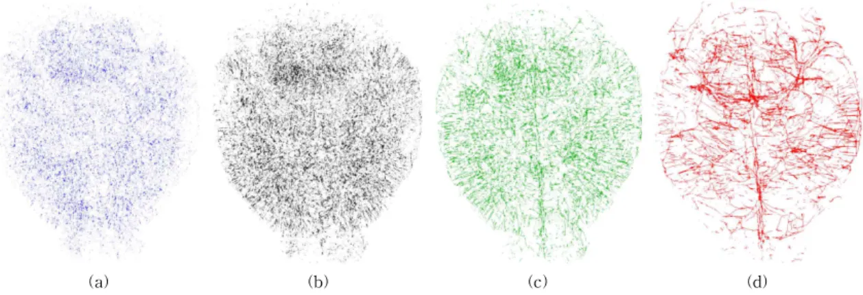
Fig. 6. Categorized vessels according to diameter size. (a) Capillaries (Diameter ≤ 10.4±0.8 µm). (b) Medium-sized vessels (10.4±0.8 µm < Diameter ≤ 20.8±1.6 µm). (c) Large-sized vessels (part1) (20.8±1.6 µm < Diameter
≤ 41.6±3.2 µm). (d) Large-sized vessels (part2) (Diameter > 41.6±3.2 µm). Transverse plane (↑: Posterior,
↓: Anterior).
관의 중심점(x, y)을 찾아 연결된 혈관 사이의 중심 점과 중심점을 서로 연결하여 혈관의 지름 크기별 전체적인 혈관 네트워크 구조를 가시화 하였다[24].
4. 실험 결과
Table 1에서 제시한 기준에 따라 혈관 지름 크기 별로 분류된 혈관의 네트워크 구조를 명확하게 구분 하기 위해 Fig. 6과 같이 4가지 색으로 가시화 하였 다. 2.2장에서 언급한 것과 같이 z축을 기준으로 연속 된 이미지에서 혈관이 서로 연결되어 있으면 그 혈관 들의 중심점을 찾고 연결하는 방법을 사용하여 x, y, z의 좌표 정보를 저장하고 있는 VTK(Visualization Toolkit) [25] 파일을 생성하였다. 이렇게 생성된 VTK 파일을 Paraview(데이터 분석 및 가시화 소프 트웨어) [26] 프로그램으로 실행하면 Fig. 6과 같이 3D 형태로 쥐 전체 뇌혈관의 지름 크기에 따른 네트 워크 구조가 완성 된다.
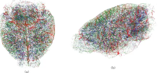
Fig. 7은 C57BL/6J 쥐 모델의 전체 뇌혈관 구조를 나타내는 그림으로 Fig. 6의 네 가지 결과를 하나로 합친 결과를 보여주고 있다. Fig. 7(a)는 횡단면을 Fig. 7(b)는 시상면을 도시하고 있으며, 모세혈관(지 름이 10.4 ± 0.8 μm 이하)은 파란색, 중간 크기의 혈관 (10.4±0.8 μm < 지름 ≤ 20.8±1.6 μm)은 검은색, 큰 크기의 혈관 부분1(20.8±1.6 μm < 지름 ≤ 41.6±3.2
μm)은 초록색으로 큰 크기의 혈관 부분2(지름 > 41.6
±3.2 μm)는 빨간색으로 혈관의 네트워크 구조를 구 분 하였다.
5. 결 론
본 논문에서는 KESM으로부터 얻은 인디아 잉크 로 염색된 쥐 전체 뇌의 혈관 이미지 데이터 세트로 부터 다양한 디지털 이미지 프로세싱 기법을 적용함 으로써 노이즈를 제거하고, 혈관의 정보만을 분류하 기 위해 최소화 임계법 기법으로 이미지를 이진화 하였다. 이렇게 이진화 된 이미지에서 혈관의 지름 크기에 따라 혈관 정보를 4단계의 기준에 따라 분류 하고, 혈관의 크기별 네트워크 구조를 시각화하여 구 분하기 위해 각기 다른 4가지 색을 적용하여 쥐의 전체 뇌혈관 네트워크 구조를 분석 하였다. 본 논문 에서의 결과는 1 μm 이하의 고해상도에서 모세혈관 (지름이 10 μm 이하)에 대한 풍부한 정보를 얻을 수 있으며, 뇌 혈관계 및 주변 대뇌의 구조에 대한 데이 터 중심의 정량적 연구에 매우 유용하게 활용될 것으 로 기대된다. 향후 연구에서는 제안된 방법보다 더 발달된 이미지 임계화 기법을 활용하여 이진화 된 이미지에서 보다 더 풍부한 양의 혈관 정보를 얻을 수 있도록 기법을 적용하고, 결과를 비교 분석 할 것 이다.
(a) (b)
Fig. 7. Distribution of vessels according to diameter size over the whole mouse brain. (a) Transverse plane (↑:
Posterior,↓: Anterior). (b) Sagittal view (←: Anterior, →: Posterior). I categorized blood vessels from capil-
laries (Diameter ≤ 10.4±0.8 µm) in blue, medium-sized vessels (10.4±0.8 µm < Diameter ≤ 20.8±1.6 µm)
in black, large-sized vessels (part1) (20.8±1.6 µm < Diameter ≤ 41.6±3.2 µm) in green, large-sized vessels
(part2) (Diameter > 41.6±3.2 µm) in red.
of Neurology, Vol. 262, No. 11, pp. 2411-2419, 2015.
[ 3 ] J.M. Wardlaw, C. Smith, and M. Dichgans,
“Mechanisms of Sporadic Cerebral Small Vessel Disease: Insights From Neuroimag- ing,” The Lancet Neurology, Vol. 12, No. 5, pp. 483-497, 2013.
[ 4 ] J.M. Wardlaw, M.S. Dennis, C.P. Warlow, and P.A. Sandercock, “Imaging Appearance of the Symptomatic Perforating Artery in Patients with Lacunar Infarction: Occlusion or Other Vascular Pathology?,” Annals of Neurology, Vol. 50, No. 2, pp. 208-215, 2001.
[ 5 ] G.E. Mead, S.C. Lewis, J.M. Wardlaw, M.S.
Dennis, and C.P. Warlow, “How Well Does the Oxfordshire Community Stroke Project Clas- sification Predict the Site and Size of the Infarct on Brain Imaging?,” Journal of Neu- rology, Neurosurgery and Psychiatry, Vol.
68, No. 5, pp. 558-562, 2000.
[ 6 ] B.H. McCormick and D.M. Mayerich, “Three- dimensional Imaging Using Knife-edge Scan- ning Microscopy,” Microscopy and Microa- nalysis, Vol. 10, No. S02, pp. 1466-1467, 2004.
[ 7 ] Y. Choe, L.C. Abbott, D. Han, P.S. Huang, J.
Keyser, J. Kwon, et al., “Knife-edge Scanning Microscopy: High-throughput Imaging and Analysis of Massive Volumes of Biological Microstructures,” High-Throughput Image Reconstruction and Analysis: Intelligent Microscopy Applications, pp. 11-37, 2008.
[ 8 ] Y. Choe, D. Mayerich, J. Kwon, D.E. Miller, J.R. Chung, C. Sung, et al., “Knife-edge Scan- ning Microscopy for Connectomics Research,”
pp. 1-11, 2011.
[10] M.J. Pesavento, C. Miller, K. Pelton, M.
Maloof, C.E. Monteith, V. Vemuri, et al.,
“Knife-edge Scanning Microscopy for Bright- field Multi-cubic Centimeter Analysis of Microvasculature,” Microscopy Today, Vol 25, No. 4, pp. 14-21, 2017.
[11] D. Mayerich, L. Abbott, and B. McCormick,
“Knife-Edge Scanning Microscopy for Imaging and Reconstruction of Three-Dimensional Anatomical Structures of the Mouse Brain,”
J ournal of Microscopy, Vol. 231, No. 1, pp.
134-143, 2008.
[12] J.R. Chung, C. Sung, D. Mayerich, J. Kwon, D.E. Miller, T. Huffman, et al., “Multiscale Exploration of Mouse Brain Microstructures Using the Knife-edge Scanning Microscope Brain Atlas,”Frontiers in Neuroinformatics, Vol 5, Article 29, pp. 1-17, 2011.
[13] J. Prewitt and M.L. Mendelsohn, “The Anal- ysis of Cell Images,”Annals of the New York Academy of Sciences, Vol. 128, No. 1, pp. 1035- 1053, 1966.
[14] J. Lee, W. An, and Y. Choe, “Mapping the Full Vascular Network in the Mouse Brain at Submicrometer Resolution,” Proceeding of 39th Annual International Conference of the IEEE Engineering in Medicine and Biology Society, pp. 3309-3312, 2017.
[15] T.H. B¨ar and J.R. Wolff, “The Formation of Capillary Basement Membranes during Internal Vascularization of the Rat’s Cerebral Cortex,” Zeitschrift f¨ur Zellforschung Und Mikroskopische Anatomie, Vol. 133, No. 2, pp.
231-248, 1972.
[16] O. Hunziker, H. Frey, and U. Schulz, “Mor- phometric Investigations of Capillaries in the Brain Cortex of the Cat,”Brain Research, Vol.
65, No. 1, pp. 1-11, 1974.
[17] M. Mato and S. Ookawara, “A Simple Method for Observation of Capillary Nets in Rat Brain Cortex,”Experientia, Vol. 35, No. 4, pp. 501- 503, 1979.
[18] N.G. Conradi, J. Engvall, and J.R. Wolff,
“Angioarchitectonics of Rat Cerebellar Cortex during Pre-and Postnatal Development,”Acta neuropathologica, Vol. 50, No. 2, pp. 131-138, 1980.
[19] H. Michaloudi, C. Batzios, I. Grivas, M.
Chiotelli, and G.C. Papadopoulos, “Develop- mental Changes in the Vascular Network of the Rat Visual Areas 17, 18 and 18a,” Brain Research, Vol. 1103, No. 1, pp. 1-12, 2006.
[20] B. Xiong, A. Li, Y. Lou, S. Chen, B. Long, J.
Peng, et al., “Precise Cerebral Vascular Atlas in Stereotaxic Coordinates of Whole Mouse Brain,” Frontiers in Neuroanatomy, Vol. 11, Article 128, pp. 1-17, 2017.
[21] MATLAB Release, The Mathworks Inc., Natick, Massachusetts, United States, 2013.
[22] R.C. Gonzalez and R.E. Woods,Image P ro- cessing Toolbox User’s Guide, The Math- works Inc., Massachusetts, United States, 2000.
[23] A. Georgantzoglou, J.D. Silva, and R. Jena,
“Image Processing with Matlab and GPU,”
MATLAB Applications for the Practical Engineer, IntechOpen, 2014.
[24] S. Lim, M.R. Nowak, and Y. Choe, “Automated Neurovascular Tracing and Analysis of the Knife-edge Scanning Microscope Rat Nissl Data Set Using a Computing Cluster,” Pro- ceeding of 38th Annual International Confer- ence of the IEEE Engineering in Medicine and Biology Society, pp. 6445-6448, 2016.
[25] W.J. Schroder, K.M. Martin, and L.S. Avila, VTK User’s Guide-VTK File Formats, Kitware, Inc., New York, United States, 2000.
[26] U. Ayachit,The Paraview Guide: A Parallel Visualization Application, Kitware, Inc., New York, United States, 2015.
[27] H.S. Yoon, N. Hewage, C.W. Moon, Y.H. Kim, and H.K. Choi, “Design of 3D Visualization Software Tool based on VTK for Manual Brain Segmentation of MRI,” Journal of Korea Multimedia Society, Vol. 8, No. 2, pp.
120-127, 2015.
이 준 석