The intensity of a singular near-tip field around the vertex of a three-dimensional notch or wedge

(1)

3 차원 놋치 및 쐐기의 응력 강도계수

이용우^† • 임세영^*

The intensity of a singular near-tip field around the vertex of a three-dimensional notch or wedge

Yongwoo Lee and Seyoung Im

Key Words : M-integral(M-적분); near-tip stress intensity(응력강도).

Abstract

Singular stress fields around three-dimensional wedges are examined, and the near-tip intensity is calculated via the two-state M-integral with the aid of the domain integral representation. A numerical example demonstrates the effectiveness and accuracy of the present scheme for computing the stress intensities of singular stresses near the generic three-dimensional wedges.

1. Introduction

The computation of the near-tip intensities of the singular fields may be rather straightforward for the two- dimensional wedges, and there are many schemes available(see Im and Kim[1] and the papers cited therein, for examples). The computation of the intensities for three-dimensional wedges is much more complicated in comparison to those of the aforementioned two- dimensional ones. There are many researchers that have discussed only the order of the stress singularities on three-dimensional wedge vertices. However, no systematic computational schemes have been reported regarding the calculation of the near-tip intensities of the singular stress fields around three-dimensional wedges, to the best of the author’s knowledge.

The purpose of the present work is to report on a numerical scheme for finding the near-tip intensities around three-dimensional wedges with the aid of the two-state M-integral. A brief review is given of the eigenfunction expansion of the solution for three- dimensional elastic wedges. The two-state M-integral is applied for calculating the near-tip intensity by utilizing the complementary relationship for the eigenvalues of the three-dimensional wedges in the sense of M-integral.

For a numerical example, we choose the three- dimensional bimaterial interface corner, which was discussed by Labossiere and Dunn[2].

2. Eigenfunction expansion of the solution for three-dimensional elastic wedges

For the purpose of analysis for stress singularities at the vertex, we introduce the eigenfunction expansion (see Benthem[3], Ghahremani and Shih[4]) for the †

Mech. Eng., KAIST, [email protected]

*Professor, Mech. Eng., KAIST, [email protected]

(2)

elastic solution, which is given in the form of the separable displacement field:

)]

; ,

~ ( 2 Re[

1

)]

; ,

~( 2 Re[

1

)]

; ,

~( 2 Re[

1

1 1 1

n n n

w r w

v r v

u r u

n n

δ φ θ µ β

δ δ

+ + +

∑

=

(1)

where r, θ and φ are the spherical coordinates with the origin at the vertex O, and (u, v, w) are the components of displacement in (r, θ, φ) directions, respectively.

Values of λ_n(=δ_n+1) , which are employed for convenience of the expression instead of δ_n+1, are called the eigenvalues and its corresponding eigenfunctions are u~_n(θ,φ;λ) , ~v_n(θ,φ;λ) and

)

; ,

~_n(θ φ λ w .

Hence, the stress singularity occurs at the origin when Re(λ_n)<1. On the other hand, the strain energy is bounded at the origin and this requires Re(λ_n)>−1/2 (boundedness of strain energy requires Re(λ_n)>0 for two-dimensional wedge vertices). However, Re(λ_n)<0 implies that the displacement fields are unbounded at r=0, which is unrealistic except for a concentrated load applied at the vertex. Therefore, we are primarily interested in eigenvalues λ_n(=δ_n+1) in the range

1 )<

Re( n

0< λ .

Let the stress and strain components in the spherical coordinates be represented by 1-D arrays as follows:

) , , , , , ( ) , , , , ,

(σ₁σ₂σ₃σ₄σ₅σ₆ = σ_rr σ_θθ σ_φφ σ_θφ σ_r_φ σ_r_θ (2a) ) 2 , 2 , 2 , , , ( ) , , , , ,

(ε₁ ε₂ ε₃ ε₄ ε₅ ε₆ = ε_rr ε_θθ ε_φφ ε_θφ ε_r_φ ε_r_θ (2b)

Material constitutive relationship is then given as

j ij

i Cε

σ = (3)

where i, j =1~6, and is the material stiffness which satisfies

Cij ji

ij C

C = .

3. Application of two-state M-integral for 3-D wedges

The M-integral is written as[5]:

∫ ⁻ ⁺ ⁻

= _S _i _i _i _i_k _k t_iu_i dS m

n x m u t n Wx

M { _, } (3)

where “S” is a closed surface. Note that W and ti indicate the strain energy density and the traction components, given as C_ijklε_ijε_kl

2

=1

W and t_i=σ_ijn_j. Furthermore is the displacement component, and m the degree of homogeneity of the strain energy density, that is, 2 for the linear elastic problem, and n the degree of freedom of the spatial dimension, e.g., n is equal to 2 for two- dimensional domains or to 3 for three-dimensional bodies. Thus the M-integral for a three-dimensional linear elastic body is rewritten as:

ui

∫ ⁻ ⁻

= _S Wx_in_i t_iu_i_jx_j t_iu_i dS

M }

2

{ _, 1 (i, j =1,2,3)

Suppose two independent elastic states, “A” and

“B”. We consider another elastic state “C” obtained by superposing the two equilibrium states “A” and “B”.

Then the above M-integral is written as

M^C =M^A+M^B+M⁽^A^,^B⁾ (4)

where the superscripts “A”, “B” and “C” indicate the aforementioned elastic states, and M⁽^A^,^B⁾ is the two- state M-integral, given as :

(3)

p A

p i B i B

p S i

A i p p B kl A ij ijkl B

A [C n x t u t u x

M⁽ ^, ⁾=∫ ^ε ^ε −( _, + _, ) dS )]

u t u t

( _i^A _i^B+ _i^B _i^A

−2

1 (5)

The integral M⁽^A^,^B⁾ results from the mutual interaction between the two elastic states “A” and “B”. This integral is referred to as the two-state M-integral in this context.

Note that M⁽^A^,^B⁾ is the conservation integral for two equilibrium states since it identically vanishes for the domains with no singularities.

To explain the application of M⁽^A^,^B⁾ for generic three-dimensional wedges, we reconsider the conical domain in Fig. 1, where each of the two surfaces and , having the outward normal vectors, cuts through the lateral surface in an arbitrary manner.

Recalling that the M-integral is dependent upon the origin of the coordinate system (x

SI

SII

SI+

SL

1, x2, x3), we take its origin at the wedge vertex. We take the closed surface where means the reverse orientation of the surface , that is, the same area but with the inside the region bounded by these surfaces, we can show the path independence of the M-integral as

L

II S

S − −S_I

SI

Fig. 1 The integral path for M-integral and two-state M-integral for three-dimensional domains.

M(S_I)=M(S_II) (6)

where M(SL) = 0 and M(- ) = -M(S ) have been used.

Furthermore, the path or surface independence of the two-state M-integral

SI

) ,B A

I

M( is apparent from the above and equation (9). That is, we have

(7) )

( )

( ⁽ ^, ⁾

) , (

II B A I B

A S M S

M =

The accurate computation of the two-state integral

) , (AB

M on the far field is possible only via a regular displacement based FEM in conjunction with the volume integral for three-dimensional domains[6]. Now utilizing the domain integral and going through some manipulation, we can reach the following expressions:

)

( _, _,

) , (

j A

j i B li j B

j V i

V

A li l B km A ij ijkm B

A [C x u x u x

M =−∫II−I ε ε − σ +σ dV q ] u u_i^B _li^B _i^A _l

A

li ) ,

2(σ +σ

−1 (8)

for three-dimensional bodies, where V and represent the domains bounded by and , and and , respectively, and indicates the region bounded by and in Fig. 1. The function

is a weight function that is defined as 1 on S

I

S

VII

SII

SI I

L

SL

, ,x₂

II V

V −

SII S_I )

(x₁ x₃ q

) , (AB

I and as 0 on SII with smooth variation between SI and SII. Note that the expression (6) and (7) indicate that M and M are conserved for an arbitrary banded volume VII –VI.

The key idea of calculating β is to utilize the path _l or surface independence property of M⁽^A^,^B⁾, as given in equation (7). Firstly, a convenient auxiliary state “B” is chosen, and the elastic field of the wedge under consideration is assigned to “A”. is then calculated semi-analytically on the

I) S

)(

, (AB

M φ

θ− domain of the spherical coordinates. We need numerical integration to 0

φ θ

r

SI

SII

VII -VI

z

SL

y

x

(4)

evaluate the resulting integral on this domain. Next, from finite element analysis we obtain on the right hand side of equation (7) with the aid of the volume integral expression (8). Then equation (7) yields

)

)(

, (

II B

A S

M

β and l

this value must be invariant with respect to the choice of the auxiliary elastic state as M^{( B}^A^, ⁾ is a bilinear functional of the two elastic states “A” and “B”.

c

δl

The present procedure now boils downs to the choice of a convenient auxiliary state “B”. For this we define a complementary eigenfield for a given eigenstate.

Let the complementary eigenvalue of an arbitrary eigenvalue δ be defined in the M-integral sense as _l follows:

δ_l +δ_l^c=−3

4. Numerical Results

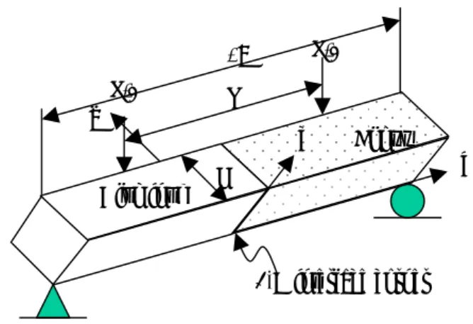
For a numerical example, we choose a three- dimensional wedge or three-dimensional bimaterial interface corner. Labossiere and Dunn[2] computed the stress singularity for three-dimensional bimaterial corners as shown in Fig. 2 using the finite element method. Furthermore, in this work, calculated was the near-tip stress intensity for this three-dimensional problem. In order to be able to compare our results with theirs, we choose the same three-dimensional interface corner as designed by Labossiere and Dunn[2] with the width h=12.5mm, and the length L=63.5mm in z-axis and the loading point distance l=76.2mm as shown in Fig.

2. The structure consists of 6061-T6 aluminum and cast West System 105-205 epoxy. Each material is isotropic with E=70.0GPa and ν=0.33 for the aluminum, and E=2.98GPa and ν=0.38 for the epoxy. The structure is the four-point bending specimen with the square cross section with h×h dimensions, where h=12.5mm as shown in Fig. 2(see Labossiere and Dunn[2] for detail).

2L P/2

P/2 l

x y Epoxy

h z Aluminum

3-D interface corner

Fig. 2 Geometric configuration of three-dimensional interface corner specimen.

Labossiere and Dunn[2] proposed the asymptotic stress and a stress intensity with the stress singularity δ for the three-dimensional interface _s corner geometry as:

) ,

~ (

~ ³ σ θ φ

σ_ij H ^Dr^δ^s _ijⁿ (9.a) )

, ,

( ₁ ₂

2 3 1 3 0

3 σ ^δ ν ν

E Y E h

H ^D = ^D ⁻^s ^D (9.b)

where r is the radius from the bimaterial interface corner, h the width as shown in Fig. 2, ( , ₁, ₂)

2

3 1 ν ν

E

D E

Y is a

nondimensional function of the elastic mismatch. The above stress intensity H³^D is equivalent to the free constant β in Eq. (1) except that their scaling may be _s different from each other due to different normalization of between Eq. (1) and (9.a). They obtained Y³^D from fitting, using the least squares approach, the asymptotic displacements fields to the full-field displacements from the finite element solution in the vicinity of the three- dimensional interface corner along the specific rays emanating from the interface corner or vertex. Note that

is the bending nominal stress that would exist at the bottom edge of a homogeneous beam of dimension

D 3

σ0

(5)

h×h under four-point loading in Fig. 18, and is written as

3 3

0 2

) ( 3

h l L

D P −

σ =

where P is the applied loading.

The finite element mesh with 3200 twenty-node solid elements and the boundary conditions of the three- dimensional bimaterial interface corner are shown in Fig.

22. Relatively refined finite element mesh is employed near the three-dimensional bimaterial interface corner.

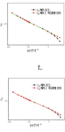
We compute the free constant β using the two-state _s M-integral and the finite element analysis using ABAQUS, as discussed in previous section. To compare the results of Labossiere and Dunn[2] with the present results, we compute the nondimensional function Y³^D in equation (9.b) as tabulated in Table 2. When the nondimensional function Y³^D is computed, the present result is obtained using the stress singularity δ =-_s 0.3586 while the result of Labossiere and Dunn[2] was obtained with the stress singularity δ =-0.351. The two _s results of the nondimensional function Y³^D are in good agreement. Using the free constant β , we obtain stress _s from the asymptotic solution of equation (1), and compare it with the result from the finite element analysis along the line θ =π/2 and φ =π/4 in Fig.

23. The finite element solution agrees well with the one term expansion (the singular term only) in the region

) (x²+y²

ρ= < 0.9mm with the width h=12.5mm.

5. Conclusions

We have examined the singular stress field around a bimaterial interface corner. Moreover, we propose a general and systematic computational scheme for computing the singular stress states near the three-

dimensional vertices with the aid of the two-state M- integral and the eigenfuntion expansion. We first verify numerically that the eigenvalues of the given three- dimensional problem satisfy the complementarity relationship, , in the three-dimensional M- integral sense. This relationship and the surface independence of the two-state M-integral are applied for extracting the near-tip intensity of the singular stress fields for three-dimensional vertices. The two numerical examples demonstrate that the present scheme is effective and accurate for computing the intensities of singular stresses near the generic three-dimensional wedges.

−3

= + _n^c

n δ

δ

Reference

(1) Im, S., and Kim, K. S, 2000, “An application of two- state M-integral for computing the intensity of the singular near-tip field for a generic wedge,” J. Mech.

Phys. of Solids, Vol. 48, pp. 129-151.

(2) Labossiere, P. E. W. and Dunn, M. L., 2001,

“Fracture initiation at three-dimensional bimaterial interface corners,” J. Mech. Phys. Solids, Vol. 49, pp.

609-634.

(3) Benthem, J. P., 1977, “State of stress at the vertex of a quarter-infinite crack in a half-space,” Int. J. Solids Struct., Vol. 13, pp. 479-492.

(4) Ghahremani, F. and Shih, C. F., 1992, “Corner singularities of three-dimensional planar interface cracks,” ASME J. Appl. Mech., Vol. 59, pp. 61-68.

(5) Knowles, J. K. and Sternberg, E., 1978, “On a class of conservation laws in a linearized and finite elatostatics,” Arch. Rat. Mech. Anal., Vol. 44, pp. 187- 211.

(6) Li F. Z., Shih F. C. and Needleman A., 1985, “A comparison of methods for calculating energy release rates,” Eng. Fract. Mech., Vol. 21, pp. 405-421.

(6)

Table 1 Complementary pairs of eigenvalues of the three-dimensional bimaterial interface corner.

(δ_n+δ_n^c =−3)

Eigenvalue -3.35770 ± i0.55264

-3.00016 -3.00005 -3.00000 -2.64139 -2.00028 -2.00022 -2.00003 -0.99997 -0.99978 -0.99972 -0.35861 0.00000 0.00005 0.00016 0.35770 ± i0.55264

Table 2 Nondimensional function Y³^D for the three- dimensional bimaterial interface corner.

Labossiere and Dunn’s

results

The present results Stress

singularity -0.351 -0.3586

Y^3D 0.303 0.302

0.01 0.1 1

σxx 0.1

ρ(=(x²+y²)^1/2) σ_xx from FEM σ_xx from asymptotic Sol.

(a)

0.01 0.1 1

0.1

σ_yy from FEM σ_yy from asymptotic Sol.

ρ(=(x²+y²)^1/2) σyy

(b)

Fig. 3 Stresses versus distance from the vertex of the interface corner along θ =π /2 and φ =π/4 for the three-dimensional aluminum/epoxy interface corner

with h=12.5mm; (a) σ_xx, (b) σ_yy.