DOI : http://dx.doi.org/10.5394/KINPR.2012.36.7.591
Prediction of Speed in Urban Freeway Having More Freight Vehicles - Based in I-696 in Michigan -
†Tae-Gon Kim, Yeon-Woo Jeong*
†Civil Engineering, Korea Maritime University, Busan 606-791, Republic. of Korea
* Civil Engineering, Korea Maritime University, Busan 606-791, Republic. of Korea
Abstract : Generally an urban freeway means a primary arterial which provides road users with a free-flow speed, except for ramp junctions during rush hours. However, most road users suffer from traffic congestion in the basic segments as well as in the ramp junctions of urban freeway during rush hours, because most road users prefer urban freeways to local roads in the urban areas. This study then intends to analyze lane traffic characteristics of urban freeway basic segments having more freight vehicles during rush hours, find the lane showing a high correlation with the segment speed between lane speeds, and finally suggest a segment-speed predictive model by the lane speed of urban freeway basic segments during rush hours.
Key words : urban freeway, lane traffic characteristics, segment speed, correlation analysis, regression modeling
†Corresponding author, [email protected] 051)410-4462
* [email protected] 051)410-4462
1. Introduction
1.1 Background
Generally, an urban freeway, as a primary arterial which is capable of carrying high traffic volumes with no more than 4 through lanes in one direction(AASHTO, 2005), must provide high-speed road users with a high level of efficiency and safety except for rush hours. In recent years urban freeways are not, however, playing a key role in high-speed road travel due to rapidly increased travel demand both at rush hours and non-rush hours. So, it is absolutely needed to improve the efficiency of use in existing urban freeways instead of building new ones.
1.2 Objectives
Most urban freeway users suffer from serious traffic congestion due to more travel demand and shorter travel length when compared to expressway. So, the purpose of this study is to suggest an appropriate segment-speed predictive model in the urban freeway basic segments having more freight vehicles. To do that, it is needed to investigate the lane traffic characteristics in urban freeway during the morning rush hour, identify the appropriate lane-speed that highly correlated with segment-speed, and finally specify the relationship between the lane-speed and
segment-speed.
1.3 Data Collection
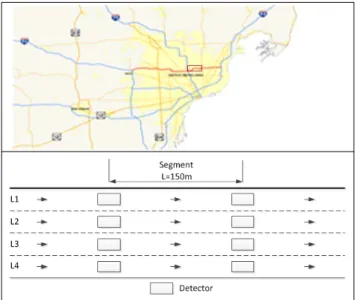
A Michigan urban freeway(I-696), a divided ground-level freeway having 4 lanes in each direction and having more freight vehicles (10% or higher) in lanes 3 and 4, was divided into 8 basic segments for data collection, as shown in Fig. 1. Its geometry is summarized in Table 1.
Fig. 1 Basic segment on urban freeway I-696
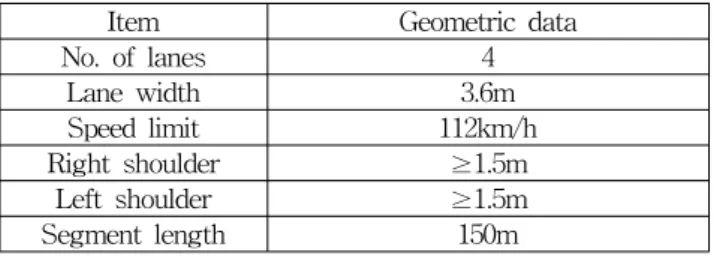
Item Geometric data
No. of lanes 4
Lane width 3.6m
Speed limit 112km/h
Right shoulder ≥1.5m
Left shoulder ≥1.5m
Segment length 150m
Table 1 Geometry of basic segment
Data collection was conducted during the morning peak period hour of 06:30 to 07:30, and a master data-set for analysis of the basic segments under study was generated every 2 minutes.
2. Analysis of traffic characteristics
2.1 Flow rate
Flow rate, as the number of vehicles per a unit time, is converted into an hourly flow rate as follows(TRB, 1975);
(1)
(2)
Where, : No. of vehicles observed for a unit time(veh)
: Observed time(2min)
: Flow rate for 2 minutes(veh/2min)
: Flow rate for 1 hour(veh/h)
There did not seem to be a significant difference in the average flow rate between segments, but there was a distinct difference between lanes except for lane 2, as shown in Fig. 2.
Segment Lane 1 Lane 2 Lane 3 Lane 4 Average 1,540
(-)
1,130 (-27%)
1,680 (+9%)
2,190 (+42%)
1,170 (-24%) Table 2 Flow rate statistics at segment(veh/h/l)
The average flow rate of lanes appeared to decrease by about 20% in lanes 1 and 4, but to increase by about 40%
in lane 3 when compared to the average flow rate of segments, as summarized in Table 2.
2.2 Speed
Speed, as the kilometers per hour, is represented by the space mean speed as follows(May, 1990);
(3)
Where, : Average speed(km/h)
: Speed of individual vehicle(km/h)
: No. of vehicles observed for a unit time(veh)
Fig. 3 Speed distribution
Similarly, the speed analysis showed that there was not a big difference in the average speed between segments, but there was a distinct difference between lanes except for lane 2, as shown in Fig. 3.
The speed analysis of lanes showed that the average speed decreased by about 10% in lanes 3 and 4, but increased by about 20% in lane 1 when compared to the average speed of segments, as summarized in Table 3.
Segment Lane 1 Lane 2 Lane 3 Lane 4
Average 94 (-)
119 (+27%)
97 (+3%)
83 (-12%)
82 (-13%) Table 3 Speed statistics at basic segment(km/h)
2.3 Density
Density, as the number of vehicles per kilometer, is computed by the reciprocal of the distance headway as follows(May, 1990);
(4)
(5)
Where, : Distance headway of individual vehicle(m)
: Average distance headway(m)
: Density(veh/km)
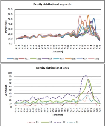
Likewise, the average density was not shown to be a significant difference between segments, but there was a considerable difference between lanes except for lane 2, as shown in Fig. 4.
The average density of lanes was shown to decrease by about 10% to 40% in lanes 1 and 4, but to increase by about 20% to 70% in lanes 2 and 3 when compared to the average density of segments, as summarized in Table 4.
Segment Lane 1 Lane 2 Lane 3 Lane 4 Average 18
(-)
13 (-28%)
23 (+28%)
33 (+83%)
16 (-11%) Table 4 Density statistics at basic segment(veh/km)
Fig. 4 Density distribution
3. Correlation analysis of traffic characteristics
3.1 Correlative characteristics of Q K
Flow rate and density appear to fall into a parabolic curve except for the outlier, as shown in Fig. 5 and 6. In particular, the maximum flow rates(Qm) and the optimal densities(KM) in the Q K curves of lanes appear to be about 2,390vph and 20vpk in lane 1, about 2,250vph and 22vpk in lane 2, about 2,990vph and 34vpk in lane 3, and finally about 1,640vph and 16vpk in lane 4, as summarized in Table 5 respectively.
Fig. 5 Q K correlative characteristics at segment
Fig. 6 Q K correlative characteristics at lanes
Qm Qm Qm Qm Qm
KM 2,140 20
KM 2,390
20
KM 2,250
22
KM 2,990
34
KM 1,640
16 Table 5 Correlation results of Q K
3.2 Correlation analysis of Q Us
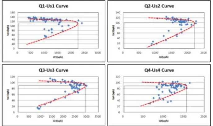
Flow rate and speed appear to fall into a parabolic curve except for the outlier, as shown in Fig. 7 and 8. In particular, the maximum flow rates(Qm) and the optimal speeds(UsM) at the Q Us curves of lanes appear to be about 2,390vph and 113kph in lane 1, about 2,250vph and 106kph in lane 2, about 2,990vph and 90vpk in lane 3, and finally about 1,640vph and 99vpk in lane 4, as summarized in Table 6 respectively.
Fig. 7 Q Us correlative characteristics at segment
Fig. 8 Q Us correlative characteristics at lanes
Qm Qm Qm Qm Qm
UsM 2,140 105
usM 2,390 113
usM 2,250
106
usM 2,990
90
usM 1,640
99 Table 6 Correlation results of Q Us
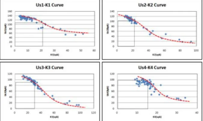
3.3 Correlation analysis of Us K
Speed and density appear to fall into a cubic curve except for the outlier, as shown in Fig. 9 and 10. In particular, the optimal speeds(UsM) and densities(KM) at the Us K curves of lanes appear to be about 113kph and 20vpk in lane 1, about 106kph and 22vpk in lane 2, about 90kph and 34vpk in lane 3, and finally about 99kph and 16vpk in lane 4, as summarized in Table 7 respectively.
Fig. 9 Us K correlative characteristics at segment
Fig. 10 Us K correlative characteristics at lanes
KM KM KM KM KM
UsM 20 105
usM 20 113
usM 22
106
usM 34
90
usM 16
99 Table 7 Correlation results of Us K
4. Model Development and Verification
4.1 Model Development
Independent variable
usi: Average speed in the lanes (i =1, 2, 3, 4) Dependent variable
Us: Average speed in the segments
Fig. 11 Variables selected for model development
Assuming that the average speed in the segments would be influenced by the lane-speeds in the segments, correlation analysis was conducted between the average speed(Us) of segments and lane-speeds(usi) in the segments. It is summarized in Table 8.
Lane-speed
Segment-speed us us us us
S1 Us r 0.858 0.969 0.954 0.968
Model CUB EXP CUB CUB
S2 Us r 0.868 0.974 0.949 0.968
Model QUA EXP CUB CUB
S3 Us r 0.891 0.979 0.961 0.950
Model EXP EXP CUB CUB
S4 Us r 0.914 0.984 0.957 0.965
Model EXP CUB CUB CUB
S5 Us r 0.934 0.977 0.968 0.978
Model CUB CUB CUB CUB
S6 Us r 0.964 0.971 0.975 0.963
Model EXP CUB CUB CUB
S7 Us r 0.953 0.970 0.967 0.956
Model EXP CUB CUB CUB
S8 Us r 0.923 0.978 0.963 0.948
Model EXP POW CUB CUB
No. of the highest r 0 6 1 1
Note: CUB is cubic model, EXP is exponential model, QUA is quadratic model, POW is power model Table 8 Correlation results of Ususiat basic segments
With the speed of lane 2(us) selected as a dependent variable and the average speed(Us) of segments selected as the independent one, segment-speed predictive models (U fus) are suggested as follows;
CUB : U × us × us × us (8) EXP : U × e×us (9) POW : U × us (10)
Where, U : Segment-speed predictive model in the segments
us: Speed of lane 2(km/h)
: Coefficients of function(=0, 1, 2, 3)
A multiple regression analysis was used to build the segment-speed predictive model, which was developed by all-possible-regression selection procedures for the purpose of identifying the important independent variables with the criteria of . In particular, multi-collinearity was avoided by the trial-and-error process.
Type Models
CUB U us us us
0.957 F-sig. 0.000
EXP U eus
0.964 F-sig. 0.000
POW U us
0.927 F-sig. 0.000
Table 9 Results of segment-speed predictive models
Thus, the segment-speed predictive model appeared as an exponential model to be in a higher explanatory power () with the speed of lane 2 than the cubic or power ones, as shown in Table 9.
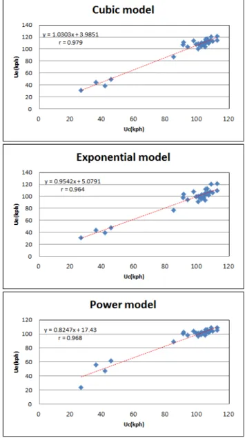
4.2 Model Verification
There were two approaches applied to ensure the validity of the models developed. One approach was to conduct the paired t-tests between the observed and expected speeds, whether the p-values were greater than the significance level (/2=0.025) or not at the 95% confidence level.
Segment Model t-value p-value Result
S5
CUB -7.366 0.000 Reject
EXP -0.692 0.494 Accept
POW -0.850 0.402 Accept
S6
CUB -7.221 0.000 Reject
EXP -0.824 0.416 Accept
POW -1.512 0.141 Accept
S7
CUB -7.510 0.000 Reject
EXP -0.953 0.348 Accept
POW -2.382 0.024 Reject
S8
CUB -7.510 0.000 Reject
EXP -0.953 0.348 Accept
POW -2.382 0.024 Reject
Table 10 Results of paired t-test
In the paired t-tests, the p-values of the exponential model (0.0.348, 0.416 and 0.494) were higher than those of the power model (0.024, 0.141 and 0.402) and of the cubic model (0.000) respectively, as shown in Table 10. Another approach was to test the utility of the regression models with traffic data that was unused. The results () of the correlation analysis were shown to be 0.951 or higher in
12. So, the exponential model proved to be very effective in predicting segment-speed in the segments.
Fig. 12 Verification at segment 5
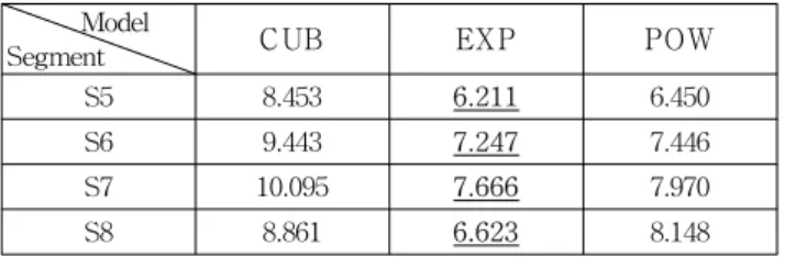
4.3 Model Evaluation
Statistics were applied to evaluate the measures of effectiveness (MOE) between the EXP model, the POW model, and the CUB model. They were to compare the root mean square error (RMSE) between the observed and expected speeds by the models. Particularly, there was less difference in the root mean square error (RMSE) of this model (6.211~7.666) than in that of the POW model (6.45 0~8.148) and the CUB model (8.453~10.095) respectively, as shown in Table 13. So, the EXP model proved to have a higher predictability than the POW and CUB models in
Model
Segment CUB EXP POW
S5 8.453 6.211 6.450
S6 9.443 7.247 7.446
S7 10.095 7.666 7.970
S8 8.861 6.623 8.148
Table 11 Results of RMSE analysis
5. Conclusions
From these traffic characteristics analyses, and the development and validation of the segment-speed predictive model in the urban freeway basic segments having more freight vehicles, the following conclusions were drawn;
1) Average speeds in the urban freeway basic segments were shown to have a higher correlation with the speed of lane 2 than lanes 3 or 4 in the basic segments 2) The exponential model proved to be suitable for
predicting the mean speed in the urban freeway basic segments with a high explanatory power and validity
It was concluded that this study needs to be continued concerning the various geometric characteristics of urban freeways having more freight vehicles for the purpose of proving the reliability of the segment-speed predictive model.
References
[1] America Association of State Highway and Transportation Officials(2004), A Policy on Geometric Design of Highways and Streets, AASHTO, Washington, D.C.
[2] Transportation Research Board(2000), Highway Capacity Manual, National Research Council, Washington, D.C.
[3] Gartner, N., Messer, C. J. and Rathi, A. K.(1997), Traffic Flow Theory; A Monograph, Special Report 165, Revised Edition, Transportation Research Board, National Research Council, Washington, D.C.
[4] Lapin, L. L.(1983), “PROBABILITY AND STATISTICS FOR MODERN ENGINEERING”, PWS Publishers, Boston, Massachusetts 02116.
Received 26 June 2012 Revised 19 September 2012 Accepted 21 September 2012