www.atmos-meas-tech.net/9/281/2016/ doi:10.5194/amt-9-281-2016
© Author(s) 2016. CC Attribution 3.0 License.
Characterization of downwelling radiance measured from a
ground-based microwave radiometer using numerical weather
prediction model data
M.-H. Ahn1, H. Y. Won1, D. Han1, Y.-H. Kim2, and J.-C. Ha2
1Department of Atmospheric Science and Engineering, Ewha Womans University, Ewha-Yeodae-Gil 52, Seodaemoon-Gu, Seoul, Republic of Korea
2National Institute of Meteorological Sciences, Korea Meteorological Administration, 33, Seohobuk-ro, Seogwipo Jeju-do, Republic of Korea
Correspondence to: M.-H. Ahn ([email protected])
Received: 11 February 2015 – Published in Atmos. Meas. Tech. Discuss.: 29 April 2015 Revised: 23 December 2015 – Accepted: 12 January 2016 – Published: 27 January 2016
Abstract. The ground-based microwave sounding radiome-ters installed at nine weather stations of Korea Meteorolog-ical Administration alongside with the wind profilers have been operating for more than 4 years. Here we apply a pro-cess to assess the characteristics of the observation data by comparing the measured brightness temperature (Tb) with reference data. For the current study, the reference data are prepared by the radiative transfer simulation with the temper-ature and humidity profiles from the numerical weather pre-diction model instead of the conventional radiosonde data. Based on the 3 years of data, from 2010 to 2012, we were able to characterize the effects of the absolute calibration on the quality of the measured Tb. We also showed that when clouds are present the comparison with the model has a high variability due to presence of cloud liquid water therefore making cloudy data not suitable for assessment of the ra-diometer’s performance. Finally we showed that differences between modeled and measured brightness temperatures are unlikely due to a shift in the selection of the center frequency but more likely due to spectroscopy issues in the wings of the 60 GHz absorption band. With a proper consideration of data affected by these two effects, it is shown that there is an ex-cellent agreement between the measured and simulated Tb. The regression coefficients are better than 0.97 along with the bias value of better than 1.0 K except for the 52.28 GHz channel which shows a rather large bias and variability of
−2.6 and 1.8 K, respectively.
1 Introduction
The potential benefits of ground-based remote sensing in-struments such as ceilometer, cloud radar, wind profiler, and passive radiometers are quite well understood and have attracted attention to the continuous efforts for an improvement (Wilczak et al., 1998; WMO, 2006; Cimini et al., 2015). Among these instruments, the ground-based microwave sounding radiometer (hereafter the radiometer) which takes measurement of the downwelling radiances (in the form of brightness temperature, Tb) in the microwave re-gion has been used to obtain the vertical information of tem-perature (T ) and humidity (q) (Cimini et al., 2006; Löhnert and Maier, 2012; Cadeddu et al., 2013). Its cost efficiency, the capability of autonomous operation, and high temporal resolution with the relatively high accuracy are the most im-portant advantages that have attracted a variety of users. For example, Knupp et al. (2009) show that the high temporal resolution data from the radiometer could resolve the rapidly changing thermodynamic structure of transitioning bound-aries, including cold fronts, gust fronts, bores, and gravity waves. It is a significant potential benefit of the radiome-ter over radiosondes to be able to detect the thermodynamic changes occurring on very short time scales, on the order of 1–10 min, which are far too short to be captured by radioson-des.
On the other hand, the radiometer is also characterized by its limited information contents which are mainly located in the lower atmosphere and by the limited vertical
resolu-tion (Löhnert et al., 2009; Candlish et al., 2012; Cadeddu et al., 2013). Due to the limitation of information contents contained within the lower atmosphere, the retrieval accu-racy of the radiometer usually decreases with increasing al-titude (Cadeddu et al., 2002; Hewison, 2007). Also, as the radiometer provides the volumetric measurement while the radiosonde measures the point value with the higher vertical resolution, the radiometer often fails to capture a sharp tem-perature change, such as the shallow inversion layer (Ware et al., 2003; Löhnert and Maier, 2012). To overcome these limitations, several efforts such as combining with satellite observation (Westwater et al., 1985; Ho et al., 2002), utiliz-ing other ground-based remote sensutiliz-ing instruments (Han and Westater, 1995; Löhnert et al., 2008, 2009), and combination with the numerical weather prediction (NWP) model (Gaus-siat et al., 2007) have been applied with a considerable im-provements, although not a consolidated approach has been established.
With the expected applications to the nowcasting and uti-lizations for the NWP model, Korea Meteorological Admin-istration (KMA) has been operating nine ground-based ra-diometers since as early as April 2009. The observation sites are selected to complement the radar wind profilers which do not provide the vertical thermodynamic information. Al-though there have been several attempts to utilize the ra-diometers in research and operational applications (Ha et al., 2010; Jeon et al., 2008; Won et al., 2009), the application has been limited, partly due to the lack of the instrument char-acterization or little understanding of the derived products. Indeed, since the beginning of the operation a thorough in-vestigation to characterize the measured data or to conduct a rigorous validation of the derived products have not been un-dertaken. Thus, for a better utilization, characterization of the instrument calibration through the analysis of the measured radiance data is highly desired.
Here, we apply a process to characterize the observation data, Tb, for a better understanding of the instrument cali-bration and to improve our understanding of the character-istics of the radiometer products. To take best advantage of the radiometers, i.e., easily operate them without human in-tervention, most of the radiometers are operated continuously without interruption except for when the regular absolute cal-ibration should be conducted. On the other hand, as there is no additional reference instrument to be used for the direct comparison, we need to find an indirect approach to charac-terize the observation data. Thus, we utilized a vicarious cal-ibration approach which compares the measured data with the reference data obtained from the simulation of a radiative transfer model (RTM). For the RTM simulation, we use the T and q profiles from the NWP models instead of radiosonde observation to overcome the limitation due to the small num-ber of collocated radiosonde data and to test feasibility of the NWP models for such a purpose. Indeed, application of the NWP model results for the characterization of the radiometer data has been used before, although it is only done for unique
occasions (Liljegren and Lesht, 1996; Cadeddu et al., 2013; Güldner, 2013).
The paper is organized as follows. Data used for the char-acterization along with the methodology including a short description of the radiative transfer model are introduced in Sect. 2. The comparison results between the measured and simulated Tbs are shown in Sect. 3, and the assessments of possible causes of the large bias between the simulated and measured Tb values are described in Sect. 4. The paper is summarized in Sect. 5 with a few lists of the planned future works.
2 Methodology and data 2.1 Methodology
One of the straight-forward approaches for the characteriza-tion of the raw data from an instrument would be the direct comparison with data from the well-characterized reference instrument. As that is not available for the radiometers in-stalled in the KMA weather stations, we use an alternative approach, by comparing the measured radiances with the simulated ones (Löhnert and Maier, 2012; Güldner, 2013). As the results of the comparison depend on the accuracy of the simulated radiances, we need a reliable RTM and the ac-curate T and q profiles which are used for the input data of RTM. Although well-characterized RTM is readily available (see below), it is not usually the case for the high quality T and q profiles, especially for a sufficiently long time period required for the correct characterization. As the main pur-pose of the radiometer installation (with the collocated wind profiler) was to fill the gaps in the network of upper weather observation, radiosonde observation is not available for the radiometer sites. Thus, here we attempt to use the T and q profiles from the NWP models (hereafter called NWP data) for the calculation of the simulated Tb. To make sure that the NWP data are accurate enough to be used as the refer-ence data, we first compare the NWP data to the T and q profiles obtained by the limited number of radiosonde obser-vations. The simulated Tbfrom the RTM simulation with the inputs from the NWP data and from the radiosonde data are also inter-compared to check the effects on the simulated Tb caused by the difference of the T and q profiles. We, then, assess the calibration characteristics by comparing the mea-sured Tb(hereafter TbM) with the simulated Tb.
2.2 Data
2.2.1 Microwave radiometer
The TbM is obtained by a ground-based microwave sound-ing radiometer manufactured by RPG Radiometer Physics GmbH (hereafter the RPG radiometer) which has been op-erating at the Changwon weather station (35.17◦N and 128.57◦E, at 37.15 m above the sea level) of South Korea
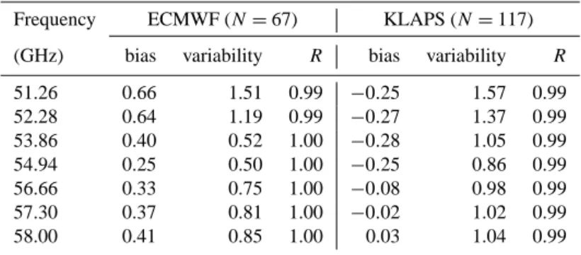
Table 1. Error statistics of the simulated Tb(TbEand TbK) obtained from the radiative transfer simulation with the input profiles of temper-ature and humidity from the NWP data, compared to the simulated Tb(TbR) with the input profiles obtained by the radiosonde. (Here and afterwards, the bias and variability are obtained from the average and standard deviation of difference between the two values, respectively). Nindicates the number of collocated NWP data with radiosonde profile data (Unit: K).
Frequency ECMWF (N = 67) KLAPS (N = 117) (GHz) bias variability R bias variability R
51.26 0.66 1.51 0.99 −0.25 1.57 0.99 52.28 0.64 1.19 0.99 −0.27 1.37 0.99 53.86 0.40 0.52 1.00 −0.28 1.05 0.99 54.94 0.25 0.50 1.00 −0.25 0.86 0.99 56.66 0.33 0.75 1.00 −0.08 0.98 0.99 57.30 0.37 0.81 1.00 −0.02 1.02 0.99 58.00 0.41 0.85 1.00 0.03 1.04 0.99
since 2010. The RPG radiometer has a total of 14 observation frequencies, 7 around the 22.24 GHz water vapor resonance line, and another 7 for the 60 GHz oxygen absorption band (RPG, 2013; also refer Table 1). The seven channels around 22.24 GHz are used for the water vapor profiling, while the seven oxygen channels are used for the temperature profil-ing. Additional products such as the total precipitable water and the cloud liquid water are also derived by the combina-tion of all 14 channels (Solheim et al., 1998; Li et al., 1997; Won et al., 2009). The Tbdata are obtained every 2–3 s with infrequent interruption for the gain calibration, looking at the internal blackbody installed inside of the RPG radiometer (RPG, 2013).
The TbM is obtained by conversion of the measured de-tector voltage using the calibration equation with the co-efficients prepared during the absolute calibration process. For the absolute calibration, four reference signals from the warm and cold targets with the addition of the noise diode signal to each target are used to derive the four calibration coefficients, including gain coefficient, non-linearity factor, background noise, and temperature of the noise diode (RPG, 2013). The warm target is internally installed blackbody and the liquid nitrogen (LN2) is used for the cold target. It is recommended to conduct the absolute calibration whenever the radiometer is newly installed, relocated, or for every 6 months. During the absolute calibration, the most serious source of uncertainty is known to come from frost formed on the surface of reflector which sends the radiation com-ing from the cold target to the radiometer. Thus, it is rec-ommended to conduct the absolute calibration with special care during the humid environment. On the other hand, the real time calibration is done by frequent observation of inter-nal blackbody and the noise diode which adds an additiointer-nal signal to the input radiance to provide a reference radiance value for the absolute calibration (RPG, 2013). During the study period, from 1 January 2010 to 31 December 2012, Tb data are continuously available except for a few occasions
in-cluding a short interruption during the early observation and during the short and regular absolute calibration periods. 2.2.2 Vertical profiles of temperature and humidity As a part of assessment test for the void upper air observation over the south-eastern part of Korea Peninsula to the weather forecasting, automatic radiosonde equipment has been oper-ated at the Changwon Weather Station since 2012. The ra-diosonde is Vaisala RS-92 GPS with known accuracy of bet-ter than 0.5 K (Nash et al., 2011; Miloshevich et al., 2009). As the radiosondes have been launched for the experimen-tal purpose, the temporal resolution is variable (from 3 to 12 h), and the observation period is also variable. For exam-ple, during the year 2012, there were two intensive obser-vation periods, one from 25 to 29 June and another from 24 to 29 August. During these periods, radiosondes were launched eight times a day, but this number was reduced to twice a day during the other observation period. Radiosonde data are available dating back to June 2012, and the number of radiosonde data used for the current study is 117. These limited number of available radiosonde data are compared with two different sets of the NWP data, one from hourly KLAPS (Korea Local-area Analysis and Prediction System; NIMR, 2012; Lee et al., 2010) analysis data and another from the 6-hourly ECMWF (European Centre for Medium-range Weather Forecasts) analysis data (Richardson et al., 2013) with the spatial resolution of 0.25◦. The NWP data are lin-early interpolated to the RPG radiometer site using the sur-rounding four grid points. For the vertical grid points, the NWP profiles are vertically interpolated to match the ra-diometer retrieval altitudes at below 10 km, while the original grid points are used for the above 10 km.
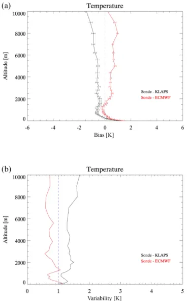
A direct comparison in terms of the bias and variability (bias and variability are obtained from the average and stan-dard deviation of the difference between the two values, re-spectively) between the available radiosonde and the NWP data are summarized in Fig. 1. The biases of the
tempera-Figure 1. The bias (a) and the variability (b) of the temperature profiles of the NWP data compared to the radiosonde data obtained from June 2012 to July 2013 (total of 117 and 67 data points for KLAPS and ECMWF, respectively). The horizontal error bar in the bias profile represents the standard deviation of mean (red and black solid lines are for the comparison between radiosonde vs. the ECMWF profile and radiosonde vs. the KLAPS data, respectively).
ture profile between the radiosonde and the NWP data are all within 1 K for at least below about 9 km except near the ground where as large as 1.5 K is found for both NWP data. Overall, the ECMWF data show a warm bias, while the KLAPS data have the cold bias, with the almost the same absolute magnitude. However, if we check the variability as shown in Fig. 1b, the ECMWF data show the smaller values. Furthermore, the ECMWF data show a quite stable variabil-ity with the altitude, while an increase with the increasing altitude is shown in the KLAPS data. Thus, from the direct comparison of the temperature profile, it is assessed that the two NWP data show a satisfactory bias characteristic in re-lation with the radiosonde uncertainty, while the variability
characteristics of the ECMWF data is better than that of the KLAPS data.
To assess the effects of these bias and variability character-istics to the simulated Tb, the RTM simulation with vertical profiles from both radiosonde and NWP data are conducted and the results are compared (see Sect. 3.1).
2.3 Radiative transfer model
For the calculation of Tb, we use the MonoRTM, a RTM that has been developed for the ARM (Atmospheric Radi-ation Measurement) program (Clough et al., 2005; Payne et al., 2011). The model can be run to simulate upwelling or downwelling radiance at the given number of monochro-matic frequencies for a range of user specified conditions in-cluding viewing geometries. Although it can incorporate the default cloud models or user-provided cloud parameters for the cloudy condition, simulations for the current study are done with the clear sky assumptions. Thus, it should be noted that the simulated Tbvalues are all considered as the clear sky Tbvalues. Utilizing the same physics as LBLRTM, the cur-rent version (V5.0) takes advantage of numerous improve-ments in the computational efficiency, the HITRAN2012 spectroscopy – except for the 60 GHz oxygen lines from Tretyakov et al. (2005), and increased flexibility (refer the home page at: http://rtweb.aer.com/monortm_frame.html for details). The accuracy for the water vapor channels, obtained from the comparison with the two frequency radiometer at an ARM sites, are known to be better than 0.28 K including both RTM and measurement error (Clough et al., 2005). On the other hand, the accuracy obtained from the comparison with the well-calibrated radiometers at the oxygen bands are estimated to have better than 1 K root mean square difference (Cadeddu et al., 2007). However, the comparison is made at the cold and dry Arctic conditions and further investigations for different climatic conditions are suggested (Cadeddu et al., 2007).
3 Comparison Results
To characterize the measured Tb, we first assess the compa-rability of the simulated Tb by using the T and q profiles obtained both from radiosonde and the NWP data at seven frequencies of the oxygen absorption band. After the assess-ment, the TbMvalues are compared with the simulated Tb val-ues. To better understand the cloud effects on TbM, compar-isons are made for both all sky and clear sky conditions. 3.1 Comparison of the simulated Tbs
Similar to the comparisons made for the T and q profiles be-tween the radiosonde and the NWP data, the simulated Tb obtained with those input profiles are compared and summa-rized in Table 1 and Fig. 2. As expected from the temperature comparisons, Tbs simulated with the ECMWF data (hereafter
Figure 2. Scatter diagram between the simulated Tbusing ECMWF data (TbE) and radiosonde data (TbR) for the lower 6 frequencies (N = 67).
TbE) show the positive bias while those with the KLAPS data (hereafter TbK) show the negative bias (Table 1). The abso-lute bias value is relatively larger at the lower frequencies, about 0.7 K, compared to the higher frequencies, about 0.4 K for EMCWF and 0.03 K for KLAPS data. Similarly, the vari-ability decreases with increasing frequency for both NWP data, having better than 1 K at most of the frequencies except at the two lower frequencies having as large as 1.6 K at the 51.26 GHz channel for the both NWP data.
As expected from the temperature comparison, the vari-ability for TbKis larger than that of TbE. In case of the corre-lation coefficients, the simulated Tbs of both NWP models show quite a good linear relationship with the radiosonde simulation, having better than 0.99 at most frequencies. Along with the bias and variability characteristics, the linear-ity characteristics between the Tbs provide a sufficient back-ground for the further utilization of the simulated Tbwith the NWP data. Thus, the characterization of the radiometer data could be extended to the cases when radiosonde observations are not available. For example, the radiometer data obtained
before June 2012 and the other eight radiometers installed at the KMA weather stations are not accompanied with the ra-diosonde observations. Furthermore, based on the bias, vari-ability, and correlation characteristics, the TbEis mainly used for the further discussions.
3.2 Measured Tbvs. simulated Tb
Here, we present the comparison results made between TbM and TbE. Table 2 summarizes the error characteristics in terms of the bias, variability, and correlation coefficients for all fre-quencies of oxygen absorption band. The comparison is ob-tained with the different data sets prepared after applying different selection criteria. For example, when no selection criteria are applied, the data set includes all of the data ob-tained during the study period (except the rain-flagged data determined by the rain sensor installed on the top of the RPG radiometer). Thus, the error statistics represent the charac-teristics the original TbM data. Seemingly, the biases look acceptable, showing the largest bias of 3.8 K at 51.26 GHz
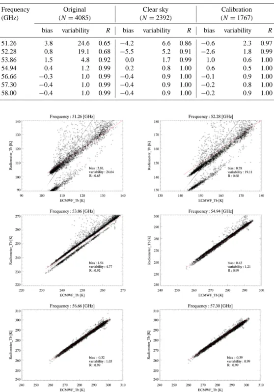
Table 2. Summary of the comparison results between TbEand TbMobtained from the data set without any screening process (original), after removing cloudy data (clear sky), and after further screening of data produced during the faulty calibration (calibration). The number of data points for the three cases are 4085, 2392, and 1767, respectively (Unit: K).
Frequency Original Clear sky Calibration
(GHz) (N = 4085) (N = 2392) (N = 1767)
bias variability R bias variability R bias variability R
51.26 3.8 24.6 0.65 −4.2 6.6 0.86 −0.6 2.3 0.97 52.28 0.8 19.1 0.68 −5.5 5.2 0.91 −2.6 1.8 0.99 53.86 1.5 4.8 0.92 0.0 1.7 0.99 1.0 0.6 1.00 54.94 0.4 1.2 0.99 0.2 0.8 1.00 0.6 0.5 1.00 56.66 −0.3 1.0 0.99 −0.4 0.9 1.00 −0.1 0.9 1.00 57.30 −0.4 1.0 0.99 −0.4 0.9 1.00 −0.2 0.8 1.00 58.00 −0.4 1.0 0.99 −0.4 0.9 1.00 −0.2 0.9 1.00
Figure 3. Comparison between the TbMand TbE(red line is the one-to-one line and N = 4063).
channel with much smaller values at the higher frequencies. However, the variability and the correlation coefficient, es-pecially at the lower three channels, show quite a large vari-ability (mainly due to the cloud contamination) and a rather
weak correlation (mainly due to the faulty absolute calibra-tion); this confirms that cloudy conditions cannot be used to characterize the TbMdata, unless the absorption of liquid
wa-Table 3. The comparison results of the different simulated Tbs and observed Tbfor clear and well-calibrated conditions for only when the radiosonde data is available (total of 26 cases).
Frequency Sonde ECMWF KLAPS
(GHz) bias variability R bias variability R bias variability R
51.26 −0.42 2.03 0.98 0.01 2.83 0.97 −1.29 2.52 0.98 52.28 −2.52 1.51 0.99 −2.00 2.10 0.99 −3.12 1.81 0.99 53.86 0.51 0.56 1.00 0.97 0.51 1.00 0.43 0.64 1.00 54.94 0.19 0.66 1.00 0.49 0.54 1.00 0.07 0.51 1.00 56.66 −0.52 0.75 1.00 −0.14 0.73 1.00 −0.66 0.84 1.00 57.30 −0.68 0.75 1.00 −0.24 0.75 1.00 −0.78 0.87 1.00 58.00 −0.73 0.82 1.00 −0.24 0.86 1.00 −0.80 0.92 1.00
ter is considered and a good estimate of the liquid water path is available.
To make sure that the comparison results are not due to the selection of the atmospheric profiles, the comparison made with other simulated Tbs with the measured Tbare shown in Table 3. Here, the error statistics are estimated using the clear and well-calibrated data obtained for when the radiosonde data are acquired. Although the total number of data matched for these conditions is only 26, the estimated error statis-tics show a comparable bias and variability characterisstatis-tics between Tbs with the radiosondes and ECMWF data, while Tbs with the KLAPS data shows a slightly larger variability, which could also be traced back to the intercomparison be-tween the simulated Tbs.
For a better understanding of the effects due to the data screening, the scatter plots between TbM and TbE for the first six frequency channels are analyzed as shown in Fig. 3 (the 58 GHz channel shows an almost identical characteris-tic with that of the 57.3 GHz channel and the results are not shown). From the scatter diagram, several interesting char-acteristics including the cloud effects are identified. First of all, channels at lower frequencies such as 51.26, 52.28, and 53.86 GHz show two distinct data groups, with one group having relatively more data points compared to the other group. The distinction is much clearer at the lowest fre-quency and diminishes with the increasing frefre-quency, be-coming indistinguishable at channels higher than 56.66 GHz. The reason for the separation turns out to be due to an appar-ent error in the absolute calibration done by using the LN2 during the early period of the instrument operation (see be-low).
Another interesting feature at these lower channels is that both the two separated groups are away from the one-to-one line (the red line) that represents a perfect match between the TbMand TbE. For example, at the 51.26 GHz channel, one denser group is closer to the one-to-one line, while another group is much further down from the one-to-one line. On the other hand, at the 52.28 GHz channel, both groups are located below the one-to-one line. It should be mentioned here that the separation and offset from the one-to-one line
also occurs at the higher frequencies such as the 54.94 GHz channel, although it is not as clearly visible as the other three lower channels. Although previous studies (Hewison et al., 2006; Löhnert and Maier, 2012) indicate this kind of offset feature is possible due to the uncertainty in the frequency assignment, detailed analysis with the simulated data given in Sect. 4 indicates the other way for the radiometer used for the current study.
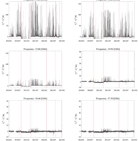
The TbM characteristics are more clearly revealed in the time series of the difference between TbMand TbE, i.e., TbM− TbE, hereafter called the Tb difference, as shown in Fig. 4. First of all, there are many data points having large positive values which are more prominent at the lower frequencies. The deviation is as high as 160 K at the 51.26 GHz chan-nel. Once again, this large positive difference is easily ex-plained by the cloud effects which add more radiation to the background clear sky radiance, resulting in the much higher TbMcompared to TbEwhich represents the clear sky condition (Turner, 2007; Cadeddu and Turner, 2011). The cloud effects decrease with the increasing frequency due to the radiation by the oxygen absorption/emission resulting in the increased contribution from the warm lower atmospheric emission to the TbM. Even with the limited effects, the cloud contami-nated data is revealed as the scattered data points in Fig. 3. Thus, for an accurate assessment of the calibration character-ization, we need to select data points free from cloud contam-ination, even at these oxygen channels. For the cloudy data screening, an algorithm using the downwelling infrared radi-ation measured by the IRT radiometer along with the surface temperature and humidity is used (Ahn et al., 2015a).
Another prominent feature from the time series shown in Fig. 4 is that the Tbdifference during a certain period, such as the period from 10 September 2010 to 31 March 2011, is much larger than the other periods. Furthermore, the differ-ence is clearly offset and discontinuous from the differdiffer-ence shown for the other time periods, implying an event that in-troduces the systematic bias and continues for a rather long time period has happened. Based on the instrument main-tenance records, the absolute calibrations were indeed per-formed in 10 September 2010 and in 31 March 2011 which
Figure 4. Time series of the difference between the TbMand TbEfor the six oxygen bands (note the different range of y axis). The red vertical bars denote the date when the absolute calibration is performed.
are exactly coincident with the points having the large dis-crepancy. Thus, it is highly suspected that the discontinuity in the error characteristics is mainly due to the uncertainty caused by the mistakes that occurred during the absolute cal-ibration done on 10 September 2010. To make sure that these kinds of error characteristics are not caused by the uncertain-ties in the simulated TbE, the time series of difference between TbM and TbK (from the KLAPS model) are also checked and it is confirmed that the same characteristics are also present (not shown). Although there is a potential way to rectify erro-neous data caused by the faulty absolute calibration, we just treat the data as it is for the further characterizations.
Overall, the error statistics improve with the progress of the data screening, especially at the lower three frequencies. As shown in Fig. 5, which shows the scatter plot between TbE and TbM for the four lower frequency channels with the data set without the cloudy and the faulty calibration period, the variability shows a significant improvement at the 51.26 (52.28) GHz channel, from 6.6 (5.2) to 2.3 K (1.8 K), along with a slight improvement of the correlation coefficient, from
0.86 (0.91) to 0.97 (0.99). At the higher frequencies, the vari-ability improvements are not that dramatic, although it shows an improvement, at all five higher channels, the variability is better than 1 K. In case of bias, although overall improve-ments at all channels are evident giving almost 0 K value, two channels, 53.86 and 54.94 GHz channels, show a slight degradation. Furthermore, the bias values at the 52.28 and 53.86 GHz channels still show a significant Tbdifference and different characteristics (positive bias at the 53.86 GHz chan-nel) compared to the previous study (Maschwitz et al., 2013), which are further described in next section.
4 Possible causes of the systematic bias
As shown in Fig. 5, even after removal of data contaminated by the faulty calibration and cloud contamination, TbM and TbEshow a clear offset from the one-to-one line with the rel-atively small variability, particularly at 52.28 and 53.86 GHz channels. The apparent systematic bias is also shown in the
Figure 5. Scatter diagram of TbEand TbMobtained after removing data with the erroneous calibration and contaminated by clouds.
comparison made with other simulated data including ra-diosonde and KLAPS analysis in addition to the other sim-ilar microwave radiometers (Hewison et al., 2006; Löhn-ert and Maier, 2012); their plausible causes are traced to center-frequency offset among other sources of uncertainties such as the band pass effect, band width effect, and so on. However, as mentioned also in Löhnert and Maier (2012) and Maschwitz et al. (2013), the RPG radiometer (Genera-tion 2) used for current study is known to have uncertainty of 1 MHz. Thus, for an assessment of the proposition of the frequency shift as the source of the systematic bias, a simple approach which searches a new frequency value that gives the least difference between TbMand TbEis applied followed by the error analysis.
To find the new frequency, we first select the clear sky TbM with free of the faulty absolute calibration to minimize uncer-tainties other than the frequency uncertainty. Then the NWP data corresponding to the observation time of the clear sky TbM are used to simulate the high-resolution (10 MHz inter-val) simulated Tbvalues as a function of frequency values. Here, it should be mentioned that the simulation resolution is coarser than the known uncertainty of 1 MHz. However, as the interested frequencies, 52.28 and 53.86 GHz, are in the valleys of absorption line centers (e.g., 52.021, 52.542, 53.066, 53.595, 54.130 GHz) where absorption is smooth with frequency due to the pressure broadening at the ground, the 10 MHz-interval simulation would give meaningful re-sults. Once the simulated Tbspectrum is prepared, the TbMis used to find the best matching frequency value which gives the least difference between the TbMand simulated Tb. As the
Table 4. The adjusted frequency for the two lower frequencies de-rived from both the ECMWF and KLAPS profiles. The adjusted fre-quency is obtained by taking averages of the frequencies that give the best match between the measured Tb(TbM) and simulated Tb (TbEor TbK). The numbers within the parentheses is averaged differ-ence and its standard deviation.
Original Adjusted Frequency (GHz)
Frequency (GHz) ECMWF KLAPS
52.28 52.24 (−0.04 ± 0.03) 52.23 (−0.05 ± 0.03) 53.86 53.88 (0.02 ± 0.01) 53.87 (0.01 ± 0.01)
simulated Tb spectrum covers all four frequency channels, the best matching frequency for each channel is simultane-ously found. Then, the difference between the known fre-quency value and newly found frefre-quency value could be con-sidered as the uncertainty in the center frequency. To increase the characterization accuracy, we use all of the selected data and also utilize both the ECMWF and KLAPS data to check the NWP model dependence of the frequency deviation. The results from all selected individual cases are used to derive the bias and variability and are summarized in Table 4.
From the Table 4, several interesting conclusions could be derived. First of all, the results from the two NWP models provide almost the same frequency shift and its variability, verifying the model inputs would not produce the system-atic bias, at least for the current study. Secondly, to remove the Tb difference between the TbM and simulated Tb, a fre-quency shift of as much as −0.04 (0.02) GHz for the 52.28
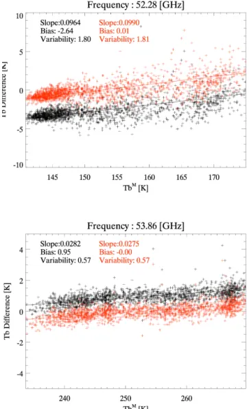
Figure 6. The Tbdifference as a function of TbM (black crosses: TbM−TbE, red crosses: TbM−Tnew) for the data set obtained af-ter removing data with faulty calibration and data contaminated by clouds. The solid lines are the best linear fit.
(53.86) GHz channel is necessary. However, the uncertainties in the estimated frequency shift (given as the variability in the Table 4) show rather large values (as much as 0.03 GHz in the 52.28 GHz), compared to the known frequency uncertain-ties of about 1 MHz (Löhnert and Maier, 2012). Thus, to fur-ther check whefur-ther the Tbdifference is indeed due to the fre-quency uncertainty, the characteristics of the newly derived TbE(or Tbnew), corresponding to the simulated Tbat the shifted frequency (for example, 52.24 GHz instead of the original 52.28 GHz), are compared to the TbM. Figure 6 shows the Tb differences, both the original Tb difference (black crosses) and the new Tbdifference (i.e., TbM−Tbnew; red crosses), as a function of the TbM. With the shifted frequency, average of the Tbdifference reduces to almost 0.0 at both channels. However, the variability and the slope (between the Tb
dif-ferences vs. TbM) do not show any meaningful change that carries an important meaning. The non-zero slope shown in the original data seemed closely related with the frequency uncertainty (Wu and Yu, 2013; Ahn et al., 2015b), and thus it could be readily argued that the Tbdifference is due to the frequency shift. In particular, when the spectral Tbis highly dependent on the frequency such as the case for the two lower channels, a small uncertainty in the center frequency pro-duces a significant uncertainty in the estimated Tb (called frequency sensitivity). Furthermore, the frequency sensitiv-ity increases with increasing target temperature, i.e. TbM, thus the frequency shift introduces the non-zero slope as shown in the original data (the black crosses). With the same argument, the frequency sensitivity of the new Tbdifference should be reduced to 0 values (see the Fig. 5 of Ahn et al., 2015b) be-cause the Tbnew is supposed to be free from the frequency uncertainty. However, as shown in Fig. 6, the red crosses have almost the same slope as the original data (the black crosses) implying the frequency shift does not remedy the large frequency sensitivity shown in the original Tb differ-ence. It should also be noted that the variability of TbM−Tbnew does not show any improvement either from the original data (from 1.80 to 1.81 K for the 52.28 GHz channel). Thus, based on these two characteristics of the Tbdifference, it should be concluded that the systematic bias shown in the two channels are not caused by the frequency uncertainty.
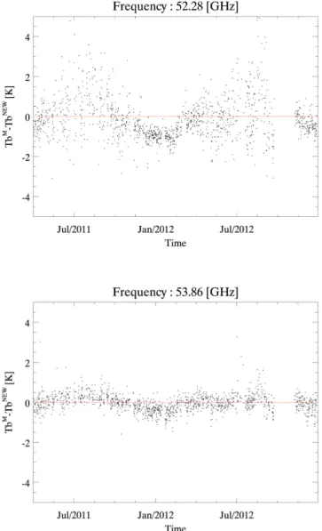
On the other hand, such a characteristic of the Tb differ-ence is also known to be introduced by the uncertainties in the spectroscopic data and/or the uncertainty in the absolute calibration of the radiometer (Cimini et al., 2004; Hewison et al., 2006; Cadeddu et al., 2007; Maschwitz et al., 2013). Al-though it is not possible to provide definitive evidence toward one cause, several aspects of the Tbdifference imply the root cause as the uncertainty in the spectroscopic data. First of all, the positive slopes shown in Fig. 6 are all consistent regard-less of the input data used for the estimation of the Tbnew, i.e. positive slopes are shown when the simulated Tbis obtained with the KLAPS data. Exactly the same characteristics of the spectral sensitivity are also shown in the similar frequency channels used for the Radiometric TP/WVP-3000 instrument (see Fig. 1 of Hewison et al., 2006). Furthermore, the time se-ries of the new Tbdifference shown in Fig. 7 shows a clear seasonality and consequently the TbMdependence (less vari-able with negative bias during the wintertime and increased variability with a positive bias during the summer time). The data affected by the faulty absolute calibration further also shows that a calibration error introduces a much different shape of the spectral sensitivity (higher value during the win-ter time in the 52.28 GHz channel, with no seasonal feature in the 53.86 GHz channel; not shown). However, as described by Maschwitz et al. (2013) the calibration accuracy also de-creases with decreasing TbM value, and thus for a detailed quantitative analysis, it is required to understand the defini-tive cause of the discrepancy.
Figure 7. Time series of TbM−Tbnew (after the frequency shift). Here, the data affected by the faulty calibration period is excluded for the comparison.
5 Summary
Nine ground-based microwave sounding radiometers of KMA have been operating since 2010 without a rigorous sensor characterization. For a better utilization of the mea-surement data, a quality assessment process on the accuracy of the radiometers has been applied. The reference measure-ments for this, the simulated downwelling radiances (or Tbs), are prepared by the radiative transfer modeling with the T and q profiles from the NWP data instead of the conven-tional radiosonde observations. Before its application, the simulated Tbwith the NWP data is validated with the sim-ulated Tbwith the limited number of radiosonde data. With the application of NWP data (from KLAPS and ECMWF), the study period could be extended, and 3 years of measure-ment data starting from the beginning of the radiometer
ob-servation at the Changwon Weather Station since 2010 are utilized.
Direct comparison between the simulated Tband measured Tb revealed the three important characteristics associated with the instrument calibration. First of all, when the absolute calibration is not properly performed, the inter-comparison between the measured and simulated Tbs reveals a clear off-set in the measured Tb, giving large values of bias and vari-ability with the quite low number of correlation coefficient. Secondly, the clouds with an appreciable optical thickness introduce a significant uncertainty in the comparison results which require a solid cloud detection algorithm for a better characterization of the instrument calibration. Finally, with the removal of the data affected by the two important degrad-ing components, the comparison results between the mea-sured and simulated Tbs agree within the previously known accuracy, better than 1 K in the bias and variability, except at the two frequency channels, the 52.28 and 53.86 GHz chan-nels which show the bias value of −2.6 and 1.0 K, respec-tively.
The proposition that uncertainty in the center frequency as the root cause of the bias is rejected by two characteristics shown in the Tbdifference. First of all, the dependence of Tb difference on the measured Tbdoes not disappear even after a new center frequency is applied to derive the Tbdifference. Secondly, the uncertainty of the necessary frequency shift to best match the measured Tband simulated Tbis way too large compared to the known frequency uncertainty. Thus, instead of the frequency uncertainty, the plausible cause for the dis-crepancy is traced to the spectroscopy data used in the prepa-ration of the simulated Tb, in view of the consistent spectral sensitivity shown with the simulated Tbs with different input profiles and results given by a different type of the radiometer along with the time series of the Tbdifference. However, to determine the definitive cause of the discrepancy a detailed quantitative analysis is required.
Even with the limitation, it is clearly shown that the sim-ulated Tbvalues using the readily available NWP data could well be used for the characterization of the radiometer. With the same application process, we plan to expand the assess-ment activities to the other radiometers being operated at other weather stations. Through the activities, overall qual-ity of the measurement data along with the identification of necessary improvements for a better utilization of the instru-ments could be derived. Also, with the microwave sounding radiometer that is manufactured by a different company and has been operating at the same weather station for a limited period of time, we would be in better position to understand the issues related with the Tbdifference, such as effects on the temperature retrieval. A similar approach, but with an ad-ditional care for the cloudy data, could be used for the wa-ter vapor channels. Finally, it should be mentioned here that even the characteristics of instrument calibration could be as-sessed with the NWP data, it would be always better to have a sufficient number of in situ observation data such as the
ra-diosonde observation. This would be more important for the evaluation of the retrieval performance.
Acknowledgements. The current work is supported by the “De-velopment and application of technology for weather forecast (NIMR-2012-B-1)” of the National Institute of Meteorological Research (NIMR). The paper is improved significantly thanks to the suggestions and critical reviews given by the anonymous reviewers and the associated editor.
Edited by: D. Cimini
References
Ahn, M.-H., Han, D., Won, H. Y., and Morris, V.: A cloud de-tection algorithm using the downwelling infrared radiance mea-sured by an infrared pyrometer of the ground-based microwave radiometer, Atmos. Meas. Tech., 8, 553–566, doi:10.5194/amt-8-553-2015, 2015a.
Ahn, M.-H., Lee, S. J., and Kim, D.: Estimation of uncertainties in the spectral response function of the water vapor channel of a me-teorological imager, Third International Conference on Remote Sensing and Geoinformation of the Environment (RSCy2015), Proc. SPIE 9535, doi:10.1117/12.2192518, 2015b.
Candlish, L. M., Raddatz, R. L., Asplin, M. G., and Barber, D. G.: Atmospheric temperature and absolute humidity profiles over the Beaufort Sea and Amundsen Gulf from a microwave radiometer, J. Atmos. Ocean. Tech., 29, 1182–1201, 2012.
Cadeddu, M. P. and Turner, D. D.: Evaluation of water permittivity models from ground-based observations of cold clouds at fre-quencies between 23 and 170 GHz, IEEE T. Geosci. Remote, 49, 2999–3008, 2011.
Cadeddu, M. P., Peckham, G. E., and Gaffard, C.: The vertical reso-lution of ground-based microwave radiometers analyzed through a multiresolution wavelet technique, IEEE Trans. Geo. Remote Sens., 40, 531–540, 2002.
Cadeddu, M. P., Payne, V. H., Clough, S. A., Cady-Pereira, K., and Liljegren, J. C.: Effect of the oxygen line-parameter modeling on temperature and humidity retrievals from ground-based mi-crowave radiometers, IEEE T. Geosci. Remote, 45, 2216–2222, 2007.
Cadeddu, M. P., Liljegren, J. C., and Turner, D. D.: The Atmo-spheric radiation measurement (ARM) program network of mi-crowave radiometers: instrumentation, data, and retrievals, At-mos. Meas. Tech., 6, 2359–2372, doi:10.5194/amt-6-2359-2013, 2013.
Cimini, D., Westwater, E. R., Han, Y., Keihm, S. J., Ware, R., Marzano, F. S., and Ciotti, P.: Atmospheric microwave radia-tive models study based on ground-based multichannel radiome-ter observations in the 20-60-Ghz band, edited by: Carrothers, D., Proceedings of the 14th ARM Science Team Meeting, Albu-querque, New Mexico, 22–26 March 2004, 1–9, 2004.
Cimini, D., Hewison, T. J., Martin, L., Güldner, J., Gaffard, C., and Marzano, F. S.: Temperature and humidity profile retrievals from ground-based microwave radiometers during TUC, Meteorol. Z., 15, 45–56, 2006.
Cimini, D., Nelson, M., Güldner, J., and Ware, R.: Forecast indices from a ground-based microwave radiometer for operational me-teorology, Atmos. Meas. Tech., 8, 315–333, doi:10.5194/amt-8-315-2015, 2015.
Clough, S. A., Shephard, M. W., Mlawer, E. J., Delamere, J. S., Ia-cono, M. J., Cady-Pereira, K., Boukabar, S., and Brown, P. D.: Atmospheric radiative transfer modeling: a summary of the AER codes, J. Quant. Spectrosc. Ra., 91, 233–244, doi:10.1016/j.jqsrt.2004.05.058, 2005.
Gaussiat, N., Hogan, R. J., and Illingworth, A. J.: Accurate liquid water path retrieval from low-cost microwave radiometers using additional information from a lidar ceilometer and operational forecast models, J. Atmos. Ocean. Tech., 24, 1562–1575, 2007. Güldner, J.: A model-based approach to adjust microwave
observa-tions for operational applicaobserva-tions: results of a campaign at Mu-nich Airport in winter 2011/2012, Atmos. Meas. Tech., 6, 2879– 2891, doi:10.5194/amt-6-2879-2013, 2013.
Ha, J.-C., Lee, J.-S., Lee, Y. H., Lee, H.-C., and Chang, D.-E.: Production of the high-resolution reanalysis data using KLAPS, Proceedings of the Spring Meeting of KMS, 29–30 April 2010, Geryong, Korea, 227–228, 2010 (in Korean with English ab-stract).
Han, Y. and Westwater, E.: Remote sensing of tropospheric water vapor and cloud liquid water by integrated ground-based sensors, J. Atmos. Ocean. Tech., 12, 1050–1059, 1995.
Hewison, T.,: 1D-VAR retrieval of temperature and humidity profiles from a ground-based microwave radiometer, IEEE T. Geosci. Remote, 45, 2163–2168, 2007.
Hewison, T., Cimini, D., Martin, L., Gaffard, C., and Nash, J.: Validating clear air absorption models using ground-based mi-crowave radiometers and vice-versa, Meteorol. Z., 15, 27–36, 2006.
Ho, S.-P., Smith, W., and Huang, H.-L.: Retrieval of atmospheric-temperature and water-vapor profiles by use of combined satel-lite and ground-based infrared spectral-radiance measurements, Appl. Optics, 41, 4057–4069, 2002.
Jeon, E.-H., Kim, Y.-H., Kim, K.-H., and Lee, H.-S.,: Operation and application guidance for the ground-based dual-band radiome-ter, Atmosphere, 18, 441–458, 2008 (in Korean with English ab-stract).
Knupp, K. R., Coleman, T., Phillips, D., Ware, R., Cimini, D., Vandenberghe, F., Vivekanandan, J., and Westwater, E.: Ground-based passive microwave profiling during dynamic weather con-ditions, J. Atmos. Ocean. Tech., 26, 1057–1073, 2009.
Lee, Y. H., Ha, J.-C., Lee, J.-S., Lee, H. C., and Chang, D.-E.: The Korean Local Reanalysis: Preliminary Result (2008–2009), The 3rd THORPEX-Asia Science Workshop and ARC-7 meeting, 3– 5 June 2010, Jeju, Korea, 2010.
Li, L., Vivekanandan, J., Chan, C., and Tsang, L.: Microwave ra-diometric technique to retrieve vapor, liquid and ice, Part I – De-velopment of a neural network-based inversion method, IEEE T. Geosci. Remote, 35, 224–236, 1997.
Liljegren, J. C. and Lesht, B. M.: Measurements of integrated wa-ter vapor and cloud liquid wawa-ter from microwave radiomewa-ters at the DOE ARM Cloud and Radiation Testbed in the US southern Great Plains, Proc. Int. Geophys. Rem. Sens. Symp., 96, 1675– 1677, 1996.
Löhnert, U. and Maier, O.: Operational profiling of tempera-ture using ground-based microwave radiometry at Payerne:
prospects and challenges, Atmos. Meas. Tech., 5, 1121–1134, doi:10.5194/amt-5-1121-2012, 2012.
Löhnert, U., Crewell, S., Krasnov, O., O’Connor, E., and Russchen-berg, H.: Advances in continuously profiling the thermodynamic state of the boundary layer: integration of measurements and methods, J. Atmos. Ocean. Tech., 25, 1251–1266, 2008. Löhnert, U., Turner, D. D., and Crewell, S.: Ground-based
tem-perature and humidity profiling using spectral infrared and mi-crowave observations. Part I: Simulated retrieval performance in clear-sky conditions, J. Appl. Meteorol. Climatol., 48, 1017– 1032, 2009.
Maschwitz, G., Löhnert, U., Crewell, S., Rose, T., and Turner, D. D.: Investigation of ground-based microwave radiometer calibra-tion techniques at 530 hPa, Atmos. Meas. Tech., 6, 2641–2658, doi:10.5194/amt-6-2641-2013, 2013.
Miloshevich, L. M., Vömel, H., Whiteman, D. N., and Leblanc, T.: Accuracy assessment and correction of Vaisala RS92 radioson-des water vapor measurements, J. Geophys. Res., 114, D11305, doi:10.1029/2008JD011565, 2009.
Nash, J., Oakley, T., Vömel, H., and Wei, L.: WMO intercomparison of high quality radiosonde systems, Yangjiang, China, 12 July–3 August 2010, WMO/TD-No. 1580, WMO, 248 pp., 2011. NIMR: Development and application of technology for weather
forecast(IV), National Institute of Meteorological Research, Seoul, Republic of Korea, Report-11-1360395-000350-09, 2012 (in Korean).
Payne, V. H., Mlawer, E. J., Cady-Pereira, K. E., and Mon-cet, J.-L.: water vapor continuum absorption in the microwave, IEEE T. Geosci. Remote, 49, 2194–2208, doi:10.1109/TGRS.2010.2091416, 2011.
Richardson, D. S., Bidlot, J., Ferranti, L., Haiden, T., Hewson, T., Janousek, M., Prates, F., and Vitart, F.: Evaluation of ECMWF forecasts, including 2012–2013 upgrades, technical memoran-dum No. 710, ECMWF, Reading, Berkshire, UK, 55 pp., 2013. RPG: Instrument Operation and Software Guide –
Princi-ple of Operation and Software Description for RPG stan-dard single-polarization radiometers, RPG, 128 pp., avail-able at http://www.radiometer-physics.de/rpg/html/docs/RPG_ MWR_STD_Software_Manual.pdf, last access: 27 April 2015.
Solheim, F., Godwin, J. R., Westwater, E. R., Han, Y., Keihm, S. J., Marsh, K., and Ware, R.: Radiometric profiling of temperature, water vapor and cloud liquid water using various inversion meth-ods, Radio Sci., 33, 393–404, 1998.
Tretyakov, M. Y., Koshelev, M. A., Dorovshikh, V. V., Makarov, D. S., and Rosenkranz , P. W.: 60-GHz oxygen band: Precise broadening and central frequencies of fine-structure lines, abso-lute absorption profile at atmospheric pressure, and revision of mixing-coefficients, J. Mol. Spectrosc., 231, 1–14, 2005. Turner, D. D.: Improved ground-based liquid water path retrievals
using a combined infrared and microwave approach, J. Geophys. Res., 112, D15204, doi:10.1029/2007JD008530, 2007.
Ware, R., Carpenter, R., Güldner, J., Liljegren, J., Nehrkorn, T., Sol-heim, F., and Vandenberghe, F.: A multichannel radiometric pro-filer of temperature, humidity, and cloud liquid, Radio Sci., 38, 8079, doi:10.1029/2002RS002856, 2003.
Westwater, E., Zhenhui, W., Grody, N., and McMillin, L.: Remote sensing of temperature profiles from a combination of observa-tions from the satellite-based Microwave Sounding Unit and the ground-based profiler, J. Atmos. Ocean. Tech., 2, 97–109, 1985. Wilczak, J. M., Gossard, E. E., Neff, W. D., and Eberhard, W. L.: Ground-based remote sensing of the atmospheric boundary layer: 25 years of progress, in: Boundary-Layer Meteorology 25th Anniversary Volume, 1970–1995, edited by: Garratt, J. R. and Taylor, P. A., Kluwer Academic Publishers, 321–349, 1998. WMO: Operational aspects of different ground-based remote sens-ing observsens-ing techniques for vertical profilsens-ing of temperature, wind, humidity and cloud structure: a review, WMO/TD-No. 1309, 37 pp., 2006.
Won, H. Y., Kim, Y.-H., and Lee, H.-S.: An application of bright-ness temperature received from a ground-based microwave ra-diometer to estimation of precipitation occurrences and rainfall intensity, Asia Pac. J. Atmos. Sci., 45, 55–69, 2009.
Wu, X. and Yu, F.: Correction for GOES imager spectral response function using GSICS – Part I: Theory, IEEE Trans. Geosci. Re-mote Sens., 51, 1215–1223, 2013.