Retinex-Based Low Contrast Image Enhancement Using Adaptive Tone-Mapping

Introduction

Previous Works

Retinex based on RGB Color Space

In Retinex theory [1], the image intensity 𝐼 is represented by the product of image reflectance 𝑅 and luminance 𝐿 given by. In the SSR algorithm [2], the convolution of the Gaussian filter, together with the input image, estimates the brightness of the image. However, the SSR algorithm has a halo artifact problem at the edges of objects and a color consistency problem caused by color shift.

To reduce halo artifact caused by the Gaussian constant c of the SSR algorithm, the MSR algorithm was proposed by Jobson [3]. For this reason, MSRCR was proposed by Jobson [4] to solve the color constancy problem of the MSR algorithm. The result of MSRCR 𝑅𝑀𝐶𝑖(𝑥, 𝑦) is given by the product of the color recovery function and the results of MSR.

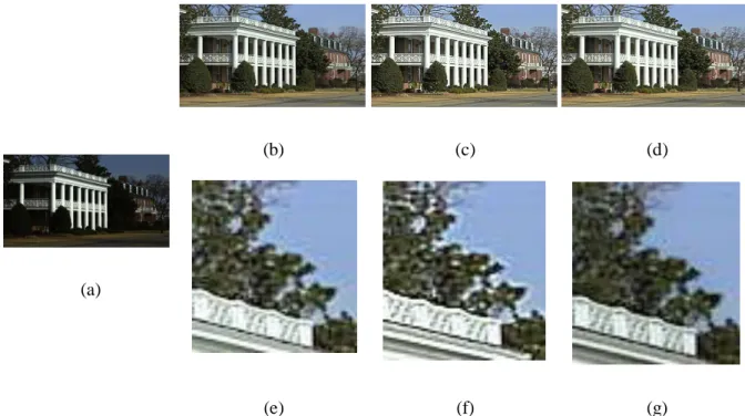
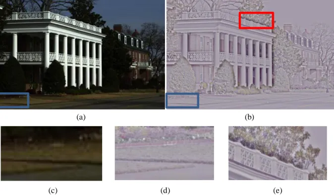
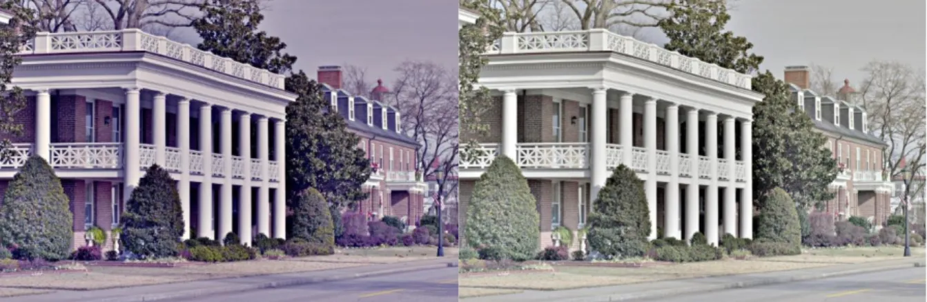
Magnified images of blue rectangles in (c) input image and (d) enhanced image. e) Magnified image of the red rectangle in the enhanced image. As shown in Figure 2.2(b), the MSRCR algorithm results in a greater improvement than MSR in terms of the color constancy problem; however, MSRCR cannot completely solve halo artifact and color constancy problems.

Retinex based on Light Channel

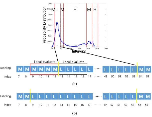
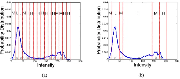
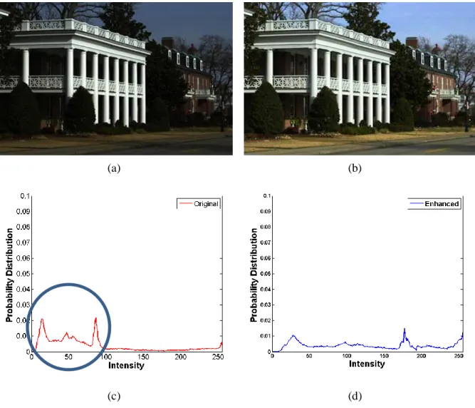
Then, we evaluate the low-contrast region of the estimated luminance using the cost function and cost labeling to enhance the image suitability. We enhance the low-contrast input image by enhancing the intensity range of the estimated luminance image 𝐿̂𝑙𝑢𝑚. More specifically, when the low-contrast image histogram and the merged estimated contrast region are labeled, as in Figure 3.5 (a), the left side of the low-contrast region is not accurately estimated.

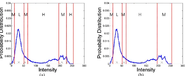
To address this, we check the local contrast region (red and black rectangles), which is located at the start or end region (shown by the yellow line) of the low-contrast region, if this region is low or no contrast. The local estimate for the low-contrast region is then obtained, as shown in Figure 3.6(a). Thus, using law-based tone mapping can improve the quality of low-contrast images.

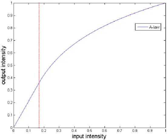
The slope of the medium-contrast region is 1 in the modified tone mapping based on the law of A. In addition, if the value of A is small, the ratio of other words in the low-contrast region is quite high, then the increasing amount in the tone mapping based on A- marriage, small. By the same token, if there is an area of ​​medium contrast in a low-contrast image, this also results in a decrease in the slope of the A-law tone mapping.

From the experimental results, we can see the importance of the location of the low-contrast region.

Proposed Algorithm

Overview

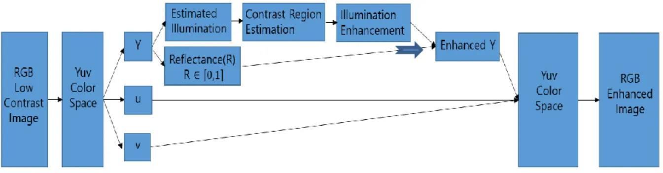
The typical Retinex-based image enhancement algorithms used a luminance channel, which is a channel that has been converted from an RGB color space, such as the Y channel in a Yuv color space or the V channel in an HSV color space. The algorithm developed in this study also uses the Y channel in a Yuv color space to preserve image color constancy. To estimate the illumination of the image, we apply an adaptive bilateral filter to the Y channel to estimate the illumination of the image.

We achieve improved illumination by applying adaptive A-law based tone mapping based on the low-contrast region estimated during the previous processing. Then we obtain an enhanced RGB image which has been converted from the enhanced Y channel and the original u and v channel.

Adaptive Bilateral Filtering

The Gaussian filter calculates the average pixel value of the adjacent pixel set and therefore often causes halo artifacts. Note that conventional bilateral filtering assigns a greater weight to neighboring pixels 𝒒(𝑢, 𝑣) that are closer to a given pixel 𝒑(𝑥, 𝑦) and that have more similar pixel values ​​to 𝒑(𝑥, 𝑦). However, in some pixels the estimated illuminance values ​​may be less than the corresponding intensity values ​​due to the smoothing nature of the applied filters.

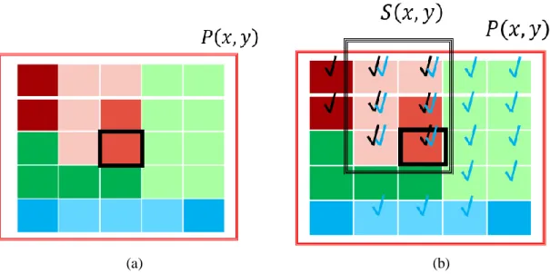
Therefore, we propose to use an adaptive bilateral filter in our algorithm to obtain a reasonable reflectance range. The red rectangle in Figure 3.2(a) represents the set of neighboring pixels for 𝒑(𝑥, 𝑦) in bilateral filtering, and the black rectangle in Figure 3.2(b) represents the set of neighboring pixels for 𝒑(𝑥, 𝑦) in ABF. The blue and black ticks in Figure 3.2(b) represent images with higher intensity and similar color.

Note that the original two-sided filtering is performed by replacing 𝑆(𝑥, 𝑦) by 𝑃(𝑥, 𝑦) in equation (3.4) above. In addition, we can further enhance detail and preserve the edge structure of the input image by smoothing neighboring pixels that have similar colors to the current pixel. However, the bilateral and guided filtering results have some halo artifacts, as shown in Figure 3.3(e) and (f).

On the other hand, the ABF result not only solves the halo artifact problem, but also preserves the naturalness of the image.

Contrast Region Partitioning

• Global Estimation
• Local Estimation
• Exception Processing

3.6) We enhance the low-contrast input image by enhancing the range of the estimated illumination image's intensity. For low-contrast image enhancement, the low-contrast region is stretched, the high-contrast region is compressed, and the middle-contrast region is preserved. So we need to determine which regions are low-contrast, medium-contrast and high-contrast to enhance the low-contrast image.

We divide the histogram, which represents the probability density of the estimated illumination of the image 𝐿̂𝑙𝑢𝑚, into 16 regions to determine the contrast region. We evaluate this value using cost-function 𝐶𝑖 and determine the label of contrast region 𝐷𝑙., as shown in Figure 3.4(a). If the labeling of the controlled region is not the same as the original labeling, the controlled region changes its labeling, and the labeling of the start or end region also changes.

If high contrast regions are set to low (0-30) or high (225-255) intensity, these regions will be absorbed into adjacent regions. This not only causes less enhancement, but also reduces the visibility quality of the final output. Furthermore, if a high-contrast region, which has a small range of about 20, is placed in a medium-intensity region, or a medium-contrast region, which has a small range of about 20, is placed between the regions that share the same label, then this region will be absorbed into an adjacent region for the same reason.

Adaptive A-law Based Tone Mapping

• A-law Based Tone Mapping
• Weighted A-law Based Tone Mapping

By doing this, we are able to stretch the dense region, while the curved part of the line (the right part of the red line) is able to compress the diffuse region. For example, if the low-contrast region is placed in a low- (Figure 3.8(a)) or high-intensity (Figure 3.8(b)) region, then the low-contrast region extends only in one direction (the direction of the red arrow in Figure 3.8(a) and (b)). Also, if a low-contrast region is placed in a mid-intensity region (Figure 3.8(c)), then the low-contrast region extends on both sides from the center of the low-contrast region.

In other words, the intensity interval in the mid-contrast region is preserved after adaptive tone mapping. Another type is a modified tonal mapping based on the A law (Figure 3.9(b)). In this type, the medium contrast area is placed between the low and high contrast areas. In this case, the applied A-law tone mapping is the same as the first line in the low and high contrast areas.

For this reason, the intensity of the mid-contrast region must either remain the same or shift while still maintaining the shape of the region. The reciprocal of the A value is determined using the degree of flatness over the entire range of the A-law function, except for the mid-contrast range. The value of the A-law function can determine the straight line segment, but it cannot control the increasing amount in intensity.

This is because the A value determines not only the degree of the even area, but also the increasing amount of the A-law function.

Final Enhanced Image

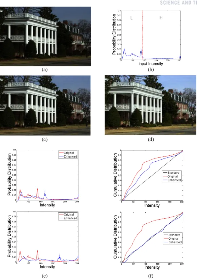
Our experiment used many low-contrast images to evaluate changes in probability distributions and cumulative distributions. Meanwhile, the low-contrast regions of Figure 4.5(a) and 4.6(a) were placed in the medium intensity, and the low-contrast region of Figure 4.7(a) was placed in the high-intensity. From these results, it can be concluded that weight A-law based tone mapping creates a greater improvement in images than conventional A-law based tone mapping in terms of visibility.

Figures 4.1 (e) and (f), 4.2 (e) and (f), 4.3 (e) and (f), and 4.4 (e) and (f) show that the A-law based tone map is more reinforcing than the conventional A-law based tone map in terms of probability distribution and cumulative distribution. Figure 4.5(c), (d), (e) and (f); 4.6 (c), (d), (e) and (f); and 4.7 (c), (d), (e), and (f) show that the conventional A-Law tone map is better than the A-law weight-based tone map in terms of visibility, but that the weight-based A-law mapping is more robust than conventional A-law-based tone mapping in terms of probability distribution and cumulative distribution. If the low-contrast region is placed in a low-intensity region, using the weighted A-law based tone map is the most suitable, especially in terms of visibility, probability distribution, and cumulative distribution.

If the low-contrast area is placed in a medium or high-intensity area, using A-law-based tone mapping is more appropriate in terms of visibility, but the weighted A-law-based tone mapping is better in terms of the other factors. Shen et al. 's algorithm [8] increases intensity to enhance low-contrast images, and this algorithm uses fixed tone mapping despite the fact that the degree of darkness varies in each image. However, similar illuminance values ​​in the same low-contrast region may be altered too much by cumulative distribution matching.

In this thesis, we proposed a low contrast image enhancement algorithm using adaptive bilateral filtering and weighted A-Law tone mapping. We solved halo artifact problem using adaptive bilateral filtering and preserved naturalness using adaptive A-law based tone mapping. Our algorithm also solved a low-contrast image enhancement problem in terms of probability and cumulative distribution.

Experimental Results

Conclusion