저작자표시

저작자표시-비영리-변경금지 2.0 대한민국 이용자는 아래의 조건을 따르는 경우에 한하여 자유롭게

l 이 저작물을 복제, 배포, 전송, 전시, 공연 및 방송할 수 있습니다. 다음과 같은 조건을 따라야 합니다:

l 귀하는, 이 저작물의 재이용이나 배포의 경우, 이 저작물에 적용된 이용허락조건 을 명확하게 나타내어야 합니다.

l 저작권자로부터 별도의 허가를 받으면 이러한 조건들은 적용되지 않습니다.

저작권법에 따른 이용자의 권리는 위의 내용에 의하여 영향을 받지 않습니다. 이것은 이용허락규약(Legal Code)을 이해하기 쉽게 요약한 것입니다.

Disclaimer

저작자표시. 귀하는 원저작자를 표시하여야 합니다.

비영리. 귀하는 이 저작물을 영리 목적으로 이용할 수 없습니다.

변경금지. 귀하는 이 저작물을 개작, 변형 또는 가공할 수 없습니다.

ᄋ ᅵ ᄋ ᅵ ᄋ

ᅵᄒ ᅡ ᆨ ᄒ ᅡ ᆨ ᄒ ᅡ ᆨᄉ ᅥ ᆨ ᄉ ᅥ ᆨ ᄉ ᅥ ᆨ ᄉ ᅡ ᄉ ᅡ ᄉ ᅡ ᄒ ᅡ ᆨ ᄒ ᅡ ᆨ ᄒ ᅡ ᆨ ᄋ ᅱ ᄋ ᅱ ᄋ ᅱ ᄂ ᅩ ᆫ ᄂ ᅩ ᆫ ᄂ ᅩ ᆫᄆ ᅮ ᆫ ᄆ ᅮ ᆫ ᄆ ᅮ ᆫ

Prediction using functional PCA with application to OES data

ᄒ ᅡ ᆷ ᄒ

ᅡ ᆷ ᄒ ᅡ ᆷ ᄉ ᅮ ᄉ ᅮ ᄉ ᅮ ᄒ ᅧ ᆼ ᄒ ᅧ ᆼ ᄒ ᅧ ᆼ ᄌ ᅮ ᄌ ᅮ ᄌ ᅮ ᄉ ᅥ ᆼ ᄉ ᅥ ᆼ ᄉ ᅥ ᆼᄇ ᅮ ᆫ ᄇ ᅮ ᆫ ᄇ ᅮ ᆫᄇ ᅮ ᆫ ᄇ ᅮ ᆫ ᄇ ᅮ ᆫᄉ ᅥ ᆨ ᄉ ᅥ ᆨ ᄉ ᅥ ᆨᄋ ᅳ ᆯ ᄋ ᅳ ᆯ ᄋ ᅳ ᆯ ᄋ ᅵ ᄋ ᅵ ᄋ ᅵ ᄋ ᅭ ᆼ ᄋ ᅭ ᆼ ᄋ ᅭ ᆼ ᄒ ᅡ ᆫ ᄒ ᅡ ᆫ ᄒ ᅡ ᆫ ᄋ ᅨ ᄋ ᅨ ᄋ ᅨ ᄎ ᅳ ᆨ ᄎ ᅳ ᆨ ᄎ ᅳ ᆨ ᄆ ᅵ ᆾ ᄆ ᅵ ᆾ ᄆ ᅵ ᆾ OES ᄃ ᅦ ᄃ ᅦ ᄃ ᅦᄋ ᅵ ᄋ ᅵ ᄋ ᅵᄐ ᅥ ᄐ ᅥ ᄐ ᅥᄅ ᅩ ᄅ ᅩ ᄅ ᅩᄋ ᅴ ᄋ ᅴ ᄋ ᅴ ᄌ ᅥ ᆨ ᄌ ᅥ ᆨ ᄌ ᅥ ᆨᄋ ᅭ ᆼ ᄋ ᅭ ᆼ ᄋ ᅭ ᆼ

2021ᄂ

ᅧ ᆫ ᄂ ᅧ ᆫ ᄂ ᅧ ᆫ

2

ᄋ ᅯ ᆯ ᄋ ᅯ ᆯ ᄋ ᅯ ᆯ

Abstract

Kyum Kim The Department of Statistics The Graduate School Seoul National University

This thesis studies the application of methods for multivariate Functional PCA (mFPCA) to longitudinal data. Functional PCA is the generalization of PCA to a setting where there are functional valued explanatory vari- ables. Existing multivariate functional data analysis methods are limited to clustering problems or cases with few explanatory variables which are not valid for actual data. In this paper, we utilize the normalization ap- proach to address the effect of variational differences between independent variables. After getting significant principal component functions, we pre- dicted a scalar value y using these functional PC scores.

Keywords: Functional Data Analysis, PCA, Normalization

Contents

1 Introduction 1

2 Functional Data Analysis (FDA) preliminaries 3

2.1 FDA . . . 3

2.2 PCA for functional data (FPCA) . . . 6

2.3 Multivariate FPCA (mFPCA) . . . 7

2.4 Normalization Method (mFPC_n) . . . 8

3 Methodology 10 3.1 Introduction . . . 10

3.2 Exploratory Data Analysis (EDA) . . . 10

3.3 FPCA . . . 11

3.4 Variable Selection . . . 11

4 Real Data Analysis 13 4.1 Data preprocessing . . . 13

4.2 Results of mFPCA . . . 15

4.2.1 Only PC1 score . . . 15 4.2.2 PC1, PC2 score . . . 16 4.3 Results of mFPCn . . . 17

5 Conclusion 20

List of Tables

List of Figures

2.1 Raw data . . . 5

4.1 Transformed data . . . 14

4.2 Design matrix . . . 15

4.3 Best subset selection 1 . . . 15

4.4 Best subset selection 2 . . . 16

4.5 Mean variations . . . 17

4.6 Normalized Data . . . 18

4.7 Best subset selection 3 . . . 18

4.8 Prediction . . . 19

4.9 Result Table . . . 19

Chapter 1

Introduction

Data from various fields are collected through a process that can be considered a functional. As the usefulness of functional data analysis has emerged, many studies in this field have recently been conducted. Examples include functional principal component analysis and functional regression.

Functional principal component analysis (FPCA) has been widely used as an effective tool of dimension reduction that minimizes loss of informa- tion. Recent studies that discussed the functional PCA method mostly focused on univariate case. These include, but not limited to, smoothed FPCA based on a roughness penalty([1],[2]). Methods for multivariate func- tional data can be found sporadically. These include pointwisely repeata- tion of classical PCA([3]), taking into variations between the components of the random functions through the normalization process([4]). However, existing multivariate functional data analysis methods are mostly limited

to clustering problems or cases with few explanatory variables which are not valid for actual data. This thesis explores a new approach that utilize multivariate functional analysis to predict scalar value.

The rest of this thesis is organized as follows. Chapter 2 briefly covers the prerequisite background of functional data analysis (FDA) and reviews the functional principal component analysis (FPCA) and multivariate ver- sion of FPCA. Chapter 4 introduces the method using multivariate func- tional principal component analysis to predict scalar value. In chapter 5, we utilize those methods to Optical Emission Spectroscopy (OES) data and predict a scalar y value using functional principal component scores. After representing the results focusing on prediction error, the paper concludes in chapter 6 with a summary and possible avenues for subsequent research.

Chapter 2

Functional Data Analysis (FDA) preliminaries

2.1 FDA

Assume that our functional data for subject i consist of discrete time pointstj, j= 1, ..., n,yi1, ..., yin. Our first job is converting these values to a computable function x(t_j) for any time point t. Because they have ob- servational errors by nature, the convention from discrete data to functions involve smoothing process. In this paper, we use roughness penalty smooth- ing method. The above process is represented by the following formula.

Functional data used in this paper (t_i, y_i), i = 1,2, ..., n satisfy following relationship:

yi =f(ti) +εi (2.1)

For basis function Bj(t), j = 1,2, ..., p, assume that:

f(t) =

p

X

j=1

β_jB_j(t) (2.2)

In this research, we utilize cubic-B spline as basis functions. The function f can be estimated by estimating the coefficients of each basis functions.

To estimate the regression coefficients, we use a penalized least squares method that minimizes:

n

X

i=1

(y_i−f(t_i))²+λ Z

f⁰⁰(s)²ds (2.3)

Estimates of functional values minimizing this could be expressed as ˆf = S_λyfor matrixS_λ, and penalty parameterλindicating complexity of smooth- ing function can be estimated by minimizing GCV:

GCV(λ) = n⁻¹SSE

(n⁻¹tr(I−Sλ))² (2.4)

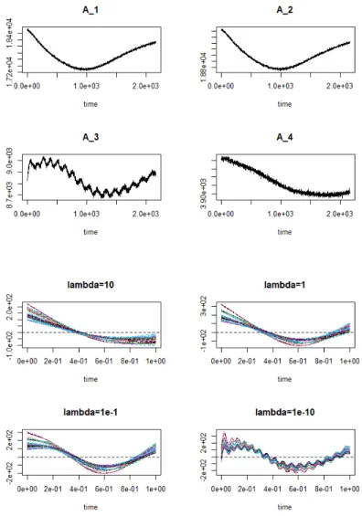
Figure 2.1: The first two rows show discrete values of the first four explanatory variables for the first subject A. The second two rows show the various version of smoothing functions corresponding the third explanatory variable of the first subject.

2.2 PCA for functional data (FPCA)

For functional data x_i(t), i = 1,2, .., N, the kth principal component score for thekth weight ξ is defined as follows:

f_ik = Z

ξ_k(s)x_i(s)ds (2.5)

We define a weighted function ξ1 as the first principal component function that maximizes the sum of the squares of the principal component scores:

maximizeN⁻¹X

i

f_i1² subject to Z

ξ₁²ds= 1 (2.6)

We then define a weighted function ξ2 perpendicular toξ1 and maximizing the sum of squares of principal component scores as the second principal component function:

maximize N⁻¹X

i

f_i2² subject to Z

ξ₂²ds= 1, Z

ξ₁ξ₂ds= 0 (2.7)

In the same way, the third and fourth principal components functions can be defined.

The following PCASSE is considered as the fitting criterion:

P CASSE =

N

X

i=1

kx_i−xˆik² (2.9)

Furthermore, it is known that the principal component weighting function minimizing the above PCASSE matches the solution that maximizes the principal component score sum.

2.3 Multivariate FPCA (mFPCA)

Consider the following bivariate case:

X_i(t) = (x_1i(t), x_2i(t)), i= 1,2, ..., N (2.10) In this case, the principal components can be defined as 2-vector ξ = (ξ^x1, ξ^x2)⁰. The principal component score is represented by the inner prod- uct of principal component function andXi, which is usually defined by the sum of the inner product of each component:

hξ₁, ξ₂i= Z

ξ₁^x1ξ₂^x1+ Z

ξ₁^x2ξ^x2₂ (2.11) We can also see this procedure as connecting function x1i(t), x2i(t) as a function and then executing univariate FPCA. The K principal component functions obtained as a result of FPCA are divided into two parts corre- sponding to x_1i(t), x_2i(t), respectively.

2.4 Normalization Method (mFPC

_n

)

Classical multivariate FPCA concatenates the multiple functions into a function to perform univariate FPCA. This can work well if components of multivariate function data are collected in the same units and have similar variations. However, when there are large variation in certain components of multivariate functional data, the classical multivariate functional PCA may not work so well.

LetD(t) =diag(v₁(t)¹/2, ..., v₁(t)¹/2), wherev_kis the variance functions of multivariate random functionsXk. Based on the Karhunen-Loeve (K-L) representation of a random function, we consider a stochastic representation for multivariate random functions:

X(t) =µ(t) +

∞

X

r=1

ξr(Dφr)(t) (2.12)

The fixed components µ_k, v_k are the mean and the variance functions, and φr r=1,2,...is a set of orthonormal basis functions satisfying

< φ_r, φ_q >=

p

X

l=1

< φ_lr, φ_lq>=δ_rq (2.13)

tation:

X(t) =µ(t) +

∞

X

r=1

ζ_rψ_r(t) (2.14)

whereψr r=1,2,...is a set of orthonormal basis functions satisfying

< ψr, ψq >=

p

X

l=1

< ψlr, ψlq>=δrq (2.15)

In this case, ζ minimize of kX−µ−P∞

r=1ζ_rψ_rk with respect to ζ_r, and could be influenced by a certain component which has relatively large value.

As a result, normalizing the data at the pre-stage allows us to obtain more stable principal component scores.

Chapter 3

Methodology

3.1 Introduction

Our goal in this paper is to predict scalar y values using multivariate functional explanatory variables. We have n objects, which we will divide into 80% training set and 20% test set. Using a training set, we will fit a regression model, which we want to use to predict the y-value of the test set. The fitting criteria for model selection is the following prediction error:

N

tern is more important than the value of the function itself, so we proceed with centralization around zero. Then identify the outline of the explana- tory variable function and check the correlation between the variables. In general, for time series data recorded in chronological order, the starting points of the variation do not match each other or the variation of the data up to a particular point may be meaningless. In this case, the data should be refined through the registration.

3.3 FPCA

Second, we obtain functional principal component (FPC) scores by con- ducting multivariate functional principal components analysis on the trans- formed data. At this point, the FPC scores are at least 80% of the total variation. For example, if the first principal component function alone can account for more than 80 percent of the total variation, we proceed with the prediction using only the first principal component. However, if the total variation is not fully explained by the first principal component func- tion alone, the prediction is carried out by obtaining the second and third principal component functions.

3.4 Variable Selection

Now divide the data into training set and test set. In a training group that is 80 percent of the total data, we can obtain an appropriate number of explanatory variables through the best subset selection function in leaps

package in R. The criterion for determining the appropriate number of explanatory variables is based on the adjusted R-squared of 0.8 or higher.

Since there is a risk of overfitting, a model with a low number of variables is prioritized when the R score exceeds 0.8. For example, if we have 20 explanatory variables, we obtain 20 principal component scores (if only the first principal component score is used) or 40 principal component scores (if up to the second principal component score is used) and choose a model with an appropriate number of explanatory variables in the training set.

Since high descriptive power in the training set does not guarantee high descriptive power in the test set, several candidate models are selected to compare the mean prediction error values in the test set. To get the mean prediction error, randomly divide into test sets and training sets 20 times to predict the y-value of the test set using the candidate models that were previously fitted, and obtain the average of the sum of prediction error.

Chapter 4

Real Data Analysis

4.1 Data preprocessing

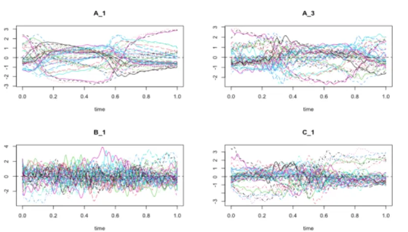
Our Optical Emission Spectroscopy (OES) data acquired during wafer etching process was collected from the three stages during the manufactur- ing process. Data at each stage were obtained in the process of projecting light from 20 wavelengths onto 43 wafers. For convenience, we will refer to five variables from the first stage as A1 to A5, and eight variables from the second stage as B1 to B9, and seven from the last stage as C1 to C6. As introduced in Chapters 2 and 3, the 20 explanatory variable functions that have undergone the smoothing and registration process are as follows.

4.2 Results of mFPCA

4.2.1 Only PC1 score

To predict the scalar value y with transformed functional data, a mul- tivariate functional PCA was performed. As a result of the functional principal component analysis, the first principal component function ex- plained 80% of the total variation and 14% of the second principal com- ponent. First, we obtained the PC1 score corresponding to each vari- ables(A1,A2,. . . ,C6) and used it to create a design matrix:

Figure 4.2: Design matrix for OES data.

The results of variable selection using the best subset selection method are as follows.

Figure 4.3: Best subset selection.

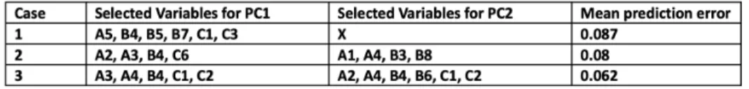
We attempt to predict using Case 6, which has the fewest number of selected variables, when the R-squared value exceeds 0.8. The variables selected in Case 6 are A5, B4, B5, B7, C1, C3. For prediction, we used the Lasso regression model and obtained 0.087 as the mean prediction error.

We also made predictions for cases 7 and 8 that use more variables, but there was little difference from the perspective of prediction error.

4.2.2 PC1, PC2 score

This time, not only PC1 score but also PC2 score were used to predict y value through a variable selection process out of 40 predictors. Figure 4.4 is the best subset selection result, and if one of the PC1 and PC2 scores is significant for one variable, the other is often not significant.

Similarly, we proceed with the prediction for cases 6,7,8, where the num- ber of selected variables is appropriate among cases where the R-squared value exceeds 0.8. As a result of the prediction, it was found that the prediction error was significantly reduced to 0.08 in case 8.

4.3 Results of mFPC

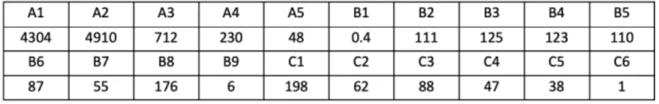
_n

For multivariate FPCA, if the variability of a particular variable is rela- tively large compared to the remaining variables, the principal component function results tend to be skewed in the direction of that variable. In this case, normalizing the data is helpful. First, we obtained 20 mean variations to examine the need for normalization.

Figure 4.5: Mean variations for 20 variables.

Given the large difference in variations for each variable, it seems mean- ingful to try the normalization method. The figure 4.6 is a visualization of some of the data that went through the normalization process.

As a result of FPCA, the first principal component function accounted for 57% of the total variation and 19% of the second principal compo- nent.Therefore, the second principal component score was decided to be used for prediction, and the best subset selection method of the Leaps

package was used to select variables.

Figure 4.6: Normalized Data

It was found that the mean prediction error was significantly reduced to 0.062 in case 11 out of several cases. In Figure 4.7, both PC1 and PC2 scores were often significant for one variable, unlike previous data. This may indicates that our method works well to divide the information that data variation has into PC1 and PC2.

Figure 4.8 is the result of predicting the remaining 9 test set after fitting the model in the above manner with 34 training set.

Figure 4.8: Prediction for test set

Figure 4.9: Result Table

Chapter 5

Conclusion

In this paper, we have developed a prediction method for multivariate longitudinal data. This method adapted multivariate functional principal component analysis (mFPCA) and normalization approach to withstand the influence of large difference between variables. Finally, this method was tested on OES data. This experiment showed that our method is effective in particular situations with large variational differences between variables.

A potentially fruitful avenue for future research is to extend our method

Bibliography

[1] Ramsey, J. and Silverman, B. Functional Data Analysis. 2nd edition.

Springer, New York, 2005.

[2] Rice, J. and Silverman, B. Estimating the mean and covariance struc- ture nonparametrically when the data are curves. Journal of the Royal Statistical Society: Series B. 53, 233-243, 1991.

[3] Silverman, B. W. Smoothed functional principal component analysis by choice of norm. Annals of Statistics. 24, 1-24, 1996.

[4] Berrendero, J. R., Justel, A. and Svarc, M. Principal components for multivariate functional data. Computational Statistics and Data Anal- ysis. 55, 2619-2634, 2011.

[5] Jeng-Min Chiou, Yu-Ting Chen and Ya-Fang Yang. Multivariate func- tional principal component analysis: A normalization approach. Statis- tica Sinica. 24, 1571-1596, 2014.

ᄀ ᅮ ᆨ ᄀ ᅮ ᆨ ᄀ ᅮ

ᆨᄆ ᅮ ᆫ ᄆ ᅮ ᆫ ᄆ ᅮ ᆫ ᄎ ᅩ ᄎ ᅩ ᄎ ᅩ ᄅ ᅩ ᆨ ᄅ ᅩ ᆨ ᄅ ᅩ ᆨ

ᄇ

ᅩᆫ 논문은

ᄃ ᅡ

변량 함

ᄉ ᅮ

형

ᄌ ᅮ

성분 분석을

ᄉ ᅵ

공간

ᄌ ᅡᄅ ᅭᄋ ᅦ

적용

ᄒ ᅡ

는 방법을 ᄐ

ᅡ

ᆷ색한

ᄃ ᅡ.

함

ᄉ ᅮ

형

ᄌ ᅮ

성분 분석은

ᄀ ᅵ

존의

ᄌ ᅮ

성분 분석을 함

ᄉ ᅮ

형

ᄌ ᅡᄅ ᅭᄋ ᅦ

적 ᄋ

ᅭ

ᆼ할

ᄉ ᅮ

있

ᄀ ᅦ

일반화한 방법

ᄋ ᅳᄅ ᅩ ᄌ ᅮᄅ ᅩ ᄉ ᅵ

공간ᄌ

ᅡᄅ ᅭ

를 분석

ᄒ ᅡ

는

ᄃ ᅦ ᄉ ᅡ

용된

ᄃ

ᅡ. ᄌ ᅵ

금

ᄁ ᅡᄌ ᅵᄋ

ᅴ 함

ᄉ ᅮ

형

ᄌ ᅮ

성분 분석은

ᄌ ᅮᄅ ᅩ

분

ᄅ ᅲ

문

ᄌ ᅦᄂ ᅡ

설명변

ᄉ ᅮᄋ

ᅴ 적은 겨

ᆼ

ᄋ ᅮᄋ ᅦ

국한

ᄒ ᅢᄉ ᅥ ᄉ ᅡ

용

ᄒ ᅢ

왔

ᄃ ᅡ

. 본 논문

ᄋ ᅦᄉ ᅥ

는 설명변

ᄉ ᅮᄀ

ᅡᆫ의 변동

ᄎ ᅡᄋ ᅵ

를

ᄀ

ᅩᄅ ᅧᄒ

ᅡᆫ 정상화 접근법을

ᄋ ᅵ

용

ᄒ ᅡᄋ ᅧ ᄌ ᅡᄅ ᅭ

를 변환

ᄒ ᅡᄀ ᅩ

,

ᄃ ᅡ

변량 함

ᄉ ᅮ

형

ᄌ ᅮ

성 ᄇ

ᅮᆫ분석을

ᄋ ᅵ

용

ᄒ ᅢ ᄋ ᅲᄋ

ᅴᄆ

ᅵᄒ

ᅡᆫ

ᄌ ᅮ

성분 점

ᄉ ᅮ

를 얻는

ᄃ ᅡ

.

ᄄ ᅩᄒ

ᅡᆫ

ᄋ ᅵ

를

ᄋ ᅵ

용

ᄒ ᅡᄋ ᅧ

,

ᄋ ᅨ

ᄎ

ᅳ

ᆨ

ᄋ ᅩᄅ ᅲ

관점

ᄋ ᅦᄉ ᅥ ᄎ

ᅬ선의측

ᄌ ᅵ

선형회귀ᄆ

ᅩ

형을 적합

ᄒ ᅡ

는

ᄀ

ᅪ정을

ᄀ ᅵ

술한

ᄃ ᅡ

.

ᄋ

ᅮᄅ ᅵ

는

ᄋ ᅵ ᄆ ᅩ

형을 식각공정

ᄌ ᅡᄅ ᅭ ᄃ ᅢᄒ ᅢ

적용한

ᄃ ᅡ

.

ᄌ ᅮ ᄌ ᅮ ᄌ

ᅮ요요요어어어: 함

ᄉ ᅮ

형

ᄌ ᅡᄅ ᅭ

분석,

ᄌ ᅮ

성분분석,정상화 ᄒ

ᅡᆨ ᄒ ᅡᆨ ᄒ

ᅡᆨ 번번번: 2019-27476