Manuscript received on September 5, 2019, Revised on September 24, Accepted on October 4, 2019
1 KEPCO Research Institute, Korea Electric Power Corporation, 105 Munji-ro Yuseong-gu, Daejeon 34056, Republic of Korea
2 Department of Mechanical Engineering, Sogang University, 35 Baekbum-ro Mapo-gu, Seoul 04107, Republic of Korea
Development of Dynamic Model of 680 MW Rated Steam Turbine and Verification and Validation of its Speed Controller
680 MW 증기터빈 동적모델 개발 및 속도제어기 검증
Inkyu Choi1†, Joohee Woo1, Gihun Son2 최인규1†, 우주희1, 손기헌2
Abstract
The steam turbine used in nuclear power plant is modeled for the purpose of verification of control system rather than the operator education. The valves, reheater and generator are modeled also and integrated into the simulator. After that, the operation data and the designed data such as heat balance diagram are utilized to identify the model parameters. It was evident that model outputs of developed simulator are very close to the measured operating ones. The simulator within dynamic model was used to verify and validate the whole control system together with field instruments. And the target plant has been operating long time.
Keywords: Steam Turbine, Model, Parameter Identification, Control
I. INTRODUCTION
In thermal or nuclear power plant, steam turbines are rotating at very high speed and the structure of them is very complex. It is always more difficult to predict the effects of proposed control system on the plant due to complexity of turbine structure [1]. Therefore, the model needs to be developed and be used for control system development and performing real-time simulations before application.
Engineers can use identification techniques widely to develop and improve dynamic or steady state models based on mathematics for which the measured operating data originated from actual system are very useful. In power plant applications, the developed mathematical models always comprise reasonable complexities that describe the system well in specific operating conditions [2].
Moreover, in such a large system as nuclear power plants, it may put them in a dangerous condition to cut turbine
control circuits when running at normal operating conditions.
Therefore, a control engineer had better to develop system models and perform verification test on the new control system before starting up the whole plant.
System identification during normal operation without any external excitation or disruption would be an ideal target, but in many cases, using operating data for identification faces limitations and external excitation is required [3].
It is introduced in this paper that mathematical models are first developed for analysis of response of control valve, steam turbine, moisture separator reheater and generator based on the physical law. And then, the measured data are used for estimating parameters for speeding up the turbine actually.
The abbreviations in this paper are represented table 1.
II. SYSTEM DESCRIPTION
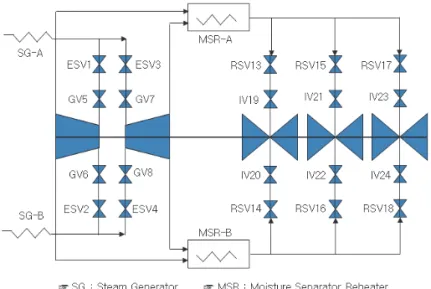
A steam turbine of a 680 MW nuclear power plant is targeted for the dynamic modeling. Fig. 1 shows the structure with nuclear steam turbine with a high pressure turbine and 3 low pressure turbine.
In addition, the system includes 2 moisture separator reheaters, and the steam generator, abbreviated as SG, produces working steam by use of heat exchange with reactor coolant.
The steam flows to each turbine are stopped or controlled by following valves.
• 4 Emergency Stop Valves: To stop steam flow to high pressure steam turbine
• 4 Governor Valves: To regulate steam flow to high pressure steam turbine
• 6 Reheater Stop Valves: To stop steam flow to low pressure steam turbine
• 6 Intercept Valves: To regulate steam flow to low pressure steam turbine
The Intercept Valves are opened fully during normal operation condition and the Governor Valves are controlling the variation turbine speed and generator output.
The high pressure steam from steam generator enter into the high pressure steam turbine. The entered steam expands and the pressure drops across the high pressure steam turbine.
The low pressure steam with low temperature is pushed into the moisture separator reheater.
The cold steam containing wet phase passes through moisture separator reheater to become dry. There are two reheaters. The very low-pressure steam from the exit of low pressure turbine is discharged into the condenser to become cool and be used in the power plant process loop again.
III. DYNAMIC MODEL DEVELOPMENT
The steam mass flow rate, pressure and enthalpy were selected as the major variables in thermal-hydraulic dynamic modeling, the parameters of which are computed by the governing equations based on such conservation laws as energy, mass and momentum. The other thermodynamic variables in dynamic model are calculated by use of the equation of state.
In a power plant with many thermal-hydraulic components including steam valves, turbines and heat exchangers, such dynamic variables as admittance, heat coefficients and pressure drops are strongly related with those of the other components.
Specially, the pressures at the inlet and outlet of each thermal-hydraulic component are determined from the operation of the matrix, which is derived by combining of the mass and momentum equations for all the other components [4]. The measured data from actually running turbine are used for calculation of turbine energy and power.
A. Steam Turbine
The steam enters the turbine through a stage nozzle from SG (Steam Generator) designed for its velocity to increase.
The pressure decrease appeared at the inlet nozzle of the steam turbine has effects on limiting the mass flow across the turbine.
A relational equation between mass flow and the pressure decrease across the turbine was developed by Stodola in 1927 [5]. At each turbine stage, the equation of pressure decrease and mass flow rate can be written as the Stodola equation.
Fig 1. Turbine configuration.
Table 1 Abbreviations
Abbreviation Description
HP/LP High Pressure/Low Pressure
SG/MSR Steam Generator/Moisture Separator Reheater ESV/GV Emergency Stop Valve/Governor Valve
RSV/IV Reheat Stop Valve/Intercept Valve Pi/ Po Pressure at inlet/at outlet
F / K Mass Flow/Admittance
y / ρi Valve Position / Steam density at inlet hi/ ho Steam enthalpy at inlet/outlet ηT/ ηgen Turbine efficiency/generator efficiency
Υ Ratio of specific heats
hos Outlet enthalpy in an isentropic process v / vi Specific volume / Specific volume at inlet
Pth Thermal power to the shaft from the steam xo Quality at outlet of MSR
hf Saturated liquid enthalpy hg Saturated vapor enthalpy V / Q Volume of MSR / heat transfer rate
N Speed of turbine and generator ωgrid/ Pelect Grid frequency / electric power
Ploss Power loss of turbine and generator IT/G Rotational inertia of turbine-generator K0, K1, K2 Loss factor
𝐹𝐹 𝐹 𝐹𝐹�𝜌𝜌�(𝑝𝑝��− 𝑝𝑝��)
𝑝𝑝� (1)
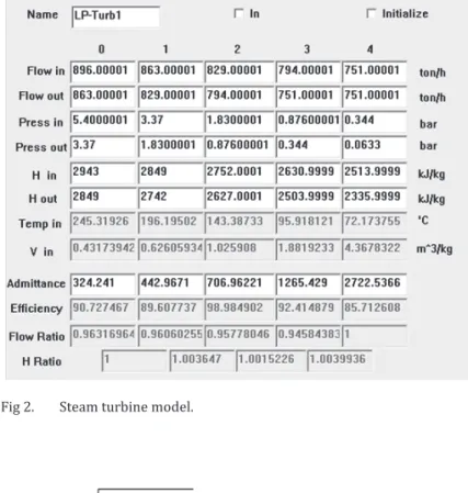
Here, admittance is calculated by the measured operating data from target power plant. The enthalpy at both the inlet and the outlet of each turbine stage is expressed by the thermodynamic of the ideal gas as the following Eq. (2).
ℎ�− ℎ�𝐹 𝜂𝜂�(ℎ��− ℎ�) (2)
where
ℎ��− ℎ�𝐹 � 𝑣𝑣�𝑝𝑝�
�
� 𝐹 − 𝛾𝛾
𝛾𝛾 − 1 𝑝𝑝�𝑣𝑣��1 − �𝑝𝑝� 𝑝𝑝��
����
� (3)
Here, hos is the enthalpy possible in an isentropic process at turbine exit, which will be computed by the state law of ideal gas as shown in Eq. (3).
The total power transferred to the rotor shaft is calculated from Eq. (4) which will be converted into electrical power after considering efficiency, friction loss and so on.
𝑃𝑃��𝐹 𝐹𝐹(ℎ�− ℎ�) (4)
Fig. 2 shows the turbine model every equation for which is depicted as follows.
B. Governor Valve
A valve is utilized to regulate the flow rate by adjusting the area of the pipe. We can express the relationship between the pressure decrease, (pi-po), and the mass flow rate, F, as follow Eq. (5).
𝐹𝐹 𝐹 𝐹𝐹𝐹𝐹(𝑦𝑦)�𝑝𝑝�− 𝑝𝑝� (5)
Here, z(y) is the function of the current valve position, y, which can be computed from the help of measured data of the power plant. No enthalpy change is assumed for the valve throttling process according to the thermodynamic principle. C. Moisture Separator Reheater
As represented in Fig. 1, 2 moisture separator reheaters (MSR) is installed between the HP turbine and the LP turbines. The MSRs reduce the moisture content of the saturated steam with moisture at the exit of the high pressure turbine.
The moisture separator reheater extracts some vapor portion of the saturated steam. We can express the mass flow rate across the reheater using the quality, x0, at the outlet of moisture separator reheater.
𝐹𝐹�𝐹 𝐹𝐹� �ℎ�− ℎ��
𝑥𝑥��ℎ�− ℎ�� (6)
The following Eq. (7), (8) and (9) shows equations of mass, energy and momentum for the reheaters.
Fig 2. Steam turbine model. Fig 3. Governor valve model.
Fig 4. Moisture separator reheater model.
II. SYSTEM DESCRIPTION
A steam turbine of a 680 MW nuclear power plant is targeted for the dynamic modeling. Fig. 1 shows the structure with nuclear steam turbine with a high pressure turbine and 3 low pressure turbine.
In addition, the system includes 2 moisture separator reheaters, and the steam generator, abbreviated as SG, produces working steam by use of heat exchange with reactor coolant.
The steam flows to each turbine are stopped or controlled by following valves.
• 4 Emergency Stop Valves: To stop steam flow to high pressure steam turbine
• 4 Governor Valves: To regulate steam flow to high pressure steam turbine
• 6 Reheater Stop Valves: To stop steam flow to low pressure steam turbine
• 6 Intercept Valves: To regulate steam flow to low pressure steam turbine
The Intercept Valves are opened fully during normal operation condition and the Governor Valves are controlling the variation turbine speed and generator output.
The high pressure steam from steam generator enter into the high pressure steam turbine. The entered steam expands and the pressure drops across the high pressure steam turbine.
The low pressure steam with low temperature is pushed into the moisture separator reheater.
The cold steam containing wet phase passes through moisture separator reheater to become dry. There are two reheaters. The very low-pressure steam from the exit of low pressure turbine is discharged into the condenser to become cool and be used in the power plant process loop again.
III. DYNAMIC MODEL DEVELOPMENT
The steam mass flow rate, pressure and enthalpy were selected as the major variables in thermal-hydraulic dynamic modeling, the parameters of which are computed by the governing equations based on such conservation laws as energy, mass and momentum. The other thermodynamic variables in dynamic model are calculated by use of the equation of state.
In a power plant with many thermal-hydraulic components including steam valves, turbines and heat exchangers, such dynamic variables as admittance, heat coefficients and pressure drops are strongly related with those of the other components.
Specially, the pressures at the inlet and outlet of each thermal-hydraulic component are determined from the operation of the matrix, which is derived by combining of the mass and momentum equations for all the other components [4]. The measured data from actually running turbine are used for calculation of turbine energy and power.
A. Steam Turbine
The steam enters the turbine through a stage nozzle from SG (Steam Generator) designed for its velocity to increase.
The pressure decrease appeared at the inlet nozzle of the steam turbine has effects on limiting the mass flow across the turbine.
A relational equation between mass flow and the pressure decrease across the turbine was developed by Stodola in 1927 [5]. At each turbine stage, the equation of pressure decrease and mass flow rate can be written as the Stodola equation.
Fig 1. Turbine configuration.
Table 1 Abbreviations
Abbreviation Description
HP/LP High Pressure/Low Pressure
SG/MSR Steam Generator/Moisture Separator Reheater ESV/GV Emergency Stop Valve/Governor Valve RSV/IV Reheat Stop Valve/Intercept Valve
Pi/ Po Pressure at inlet/at outlet F / K Mass Flow/Admittance
y / ρi Valve Position / Steam density at inlet hi/ ho Steam enthalpy at inlet/outlet ηT/ ηgen Turbine efficiency/generator efficiency
Υ Ratio of specific heats
hos Outlet enthalpy in an isentropic process v / vi Specific volume / Specific volume at inlet
Pth Thermal power to the shaft from the steam xo Quality at outlet of MSR
hf Saturated liquid enthalpy hg Saturated vapor enthalpy V / Q Volume of MSR / heat transfer rate
N Speed of turbine and generator ωgrid/ Pelect Grid frequency / electric power
Ploss Power loss of turbine and generator IT/G Rotational inertia of turbine-generator K0, K1, K2 Loss factor
𝐹𝐹 𝐹 𝐹𝐹�𝜌𝜌�(𝑝𝑝��− 𝑝𝑝��)
𝑝𝑝� (1)
Here, admittance is calculated by the measured operating data from target power plant. The enthalpy at both the inlet and the outlet of each turbine stage is expressed by the thermodynamic of the ideal gas as the following Eq. (2).
ℎ�− ℎ�𝐹 𝜂𝜂�(ℎ��− ℎ�) (2)
where
ℎ��− ℎ�𝐹 � 𝑣𝑣�𝑝𝑝�
�
� 𝐹 − 𝛾𝛾
𝛾𝛾 − 1 𝑝𝑝�𝑣𝑣��1 − �𝑝𝑝� 𝑝𝑝��
����
� (3)
Here, hos is the enthalpy possible in an isentropic process at turbine exit, which will be computed by the state law of ideal gas as shown in Eq. (3).
The total power transferred to the rotor shaft is calculated from Eq. (4) which will be converted into electrical power after considering efficiency, friction loss and so on.
𝑃𝑃��𝐹 𝐹𝐹(ℎ�− ℎ�) (4)
Fig. 2 shows the turbine model every equation for which is depicted as follows.
B. Governor Valve
A valve is utilized to regulate the flow rate by adjusting the area of the pipe. We can express the relationship between the pressure decrease, (pi-po), and the mass flow rate, F, as follow Eq. (5).
𝐹𝐹 𝐹 𝐹𝐹𝐹𝐹(𝑦𝑦)�𝑝𝑝�− 𝑝𝑝� (5)
Here, z(y) is the function of the current valve position, y, which can be computed from the help of measured data of the power plant. No enthalpy change is assumed for the valve throttling process according to the thermodynamic principle.
C. Moisture Separator Reheater
As represented in Fig. 1, 2 moisture separator reheaters (MSR) is installed between the HP turbine and the LP turbines.
The MSRs reduce the moisture content of the saturated steam with moisture at the exit of the high pressure turbine.
The moisture separator reheater extracts some vapor portion of the saturated steam. We can express the mass flow rate across the reheater using the quality, x0, at the outlet of moisture separator reheater.
𝐹𝐹�𝐹 𝐹𝐹� �ℎ�− ℎ��
𝑥𝑥��ℎ�− ℎ�� (6)
The following Eq. (7), (8) and (9) shows equations of mass, energy and momentum for the reheaters.
Fig 2. Steam turbine model. Fig 3. Governor valve model.
Fig 4. Moisture separator reheater model.
𝑉𝑉𝑑𝑑𝑑𝑑
𝑑𝑑𝑑𝑑 = 𝐹𝐹�− 𝐹𝐹� (7)
𝑑𝑑𝑉𝑉𝑑𝑑𝑑�
𝑑𝑑𝑑𝑑 = 𝐹𝐹�(𝑑�− 𝑑�) + 𝑄𝑄 (8)
𝐹𝐹 = 𝐹𝐹�𝑑𝑑(𝜌𝜌�− 𝜌𝜌�) (9)
Here, V is the volume of the moisture separator reheater and Q is the heat transfer rate.
D. Generator
Since a generator is coupled with the system grid, the generator produces electrical power based on the kinetic energy of turbine shaft. However, when it is off the grid, the thermal power to the turbine from the steam generator increases the speed of the rotor until it balances with friction loss plus windage loss. This dynamic model can be expressed as
On-grid: 𝑁𝑁 = 60𝑁𝑁����
𝑃𝑃�����= 𝜂𝜂��(𝑃𝑃��− 𝑃𝑃����) (10) Off-grid: 𝑃𝑃�����= 0
𝐼𝐼�/������= (𝑃𝑃��− 𝑃𝑃����) (11) The loss power can be totally expressed as
𝑃𝑃����= 𝐹𝐹�+ 𝐹𝐹�𝑁𝑁 + 𝐹𝐹�𝑁𝑁� (12) Here, the coefficients are determined from the operating data.
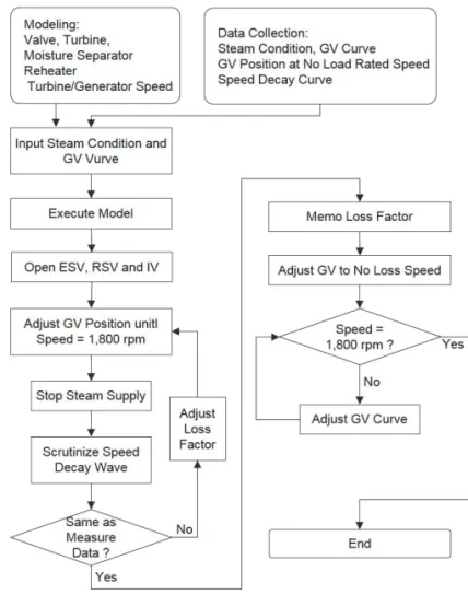
IV. PARAMETER ESTIMATION
The pressure and temperature of steam, the pressure and temperature in condenser are parameters to be decided by use of such design data as the heat balance diagram. The HP steam condition is 46 bar and 2,900 kcal/kg. The condenser condition is 0.05 bar and 32.8°C. The procedure for parameter estimation is shown in Fig. 6.
The other important element for steam flow calculation is valve characteristic curve. The natural decay curve for turbine speed is used to calculate the power loss, inertia, friction, windage loss and the positions of both the GVs an IVs at no load rated speed.
In Fig. 7, the vertical axis shows the decaying speed, the rated of which is 1,800 rpm and the horizontal axis represent the elapsed time the duration of which is about 70 minutes.
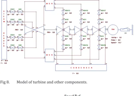
Fig 8. shows the integrated dynamic model of steam header, emergency stop valve, governor valve, high pressure turbine, moisture separator reheater, reheater stop valve, intercept valve, low pressure turbine and generator.
Fig 5. Generator model.
Fig 6. Procedure of parameter estimation.
V. ALGORITHM OF SPEED CONTROL
The newly developed digital control system which replaced old analog one contains speed control algorithm which is closely described in Fig. 9. The velocity is produced from ramp block at a certain rate depending on operator's selection.
Speed Set means an operator selected target speed whose pre-defined values are Closed, 200, 400, 800, 1,500 and 1,800 rpm.
Speed Ref Rate has meaning of the acceleration rate whose pre-defined values are 0, 40, 120 and 360 rpm/min. If the operator selects "Hold", the turbines cannot accelerate because the rate is the same as 0rpm/min. The function of ramp block automatically calculates Speed Ref according to the selected value.
The developed controller in the simulation is a simple proportional controller which is digital type with 5msec execution time. And the original controller in the actual power plant is the same proportional one which is analog type with operational amplifier and integrated circuit devices.
The digital type controller has strong points in the convenience of its use and weak points in the performance of controllability rather than analog one.
A. GV control
In Fig. 9, Kp∆F is decided by a speed error(∆F) and gain of proportional controller. Kp∆F goes up when an actual speed is smaller than speed Ref and GVs are more opened by increased GVR then the actual turbine speed increased. GVR is proportional to Kp∆F and controls all the GVs during speed up.
B. IV control
In Fig. 9, the GV controls the turbine speed according to
the following relationship.
GVR = 𝐾𝐾�Δ𝐹𝐹 (13)
The relationship between GV position and IV position is as follows.
IVR = GVR × 2.0 + 100% (14)
Eq. (14) means that 6 IVs must be fully open, even if the 4 GVs is at its fully closed position at the beginning of speed up, for all 4 GVs to control turbine speed from turning gear speed to some target speed. The bias 100% helps the 6 IVs to pass every steam which flow from 4 GVs through high pressure steam turbine and moisture separator reheater.
So, IV is controlled by IVR as following equation.
IVR = 𝐾𝐾�Δ𝐹𝐹 × 2.0 + 100% (15)
VI. SIMULATION
The simulation test can be performed only after the newly developed control system is installed in the field completely. All of the control signals can be confirmed
Fig 7. Natural speed decay.
Fig 8. Model of turbine and other components.
Fig 9. Overview of speed control algorithm. The parameters and variables used here are as follows.
Kp: Proportional Gain of Controller ∆F: Speed Error
GVR: Governor Valve Reference IVR: Intercept Valve Reference
𝑉𝑉𝑑𝑑𝑑𝑑
𝑑𝑑𝑑𝑑 = 𝐹𝐹�− 𝐹𝐹� (7)
𝑑𝑑𝑉𝑉𝑑𝑑𝑑�
𝑑𝑑𝑑𝑑 = 𝐹𝐹�(𝑑�− 𝑑�) + 𝑄𝑄 (8)
𝐹𝐹 = 𝐹𝐹�𝑑𝑑(𝜌𝜌�− 𝜌𝜌�) (9)
Here, V is the volume of the moisture separator reheater and Q is the heat transfer rate.
D. Generator
Since a generator is coupled with the system grid, the generator produces electrical power based on the kinetic energy of turbine shaft. However, when it is off the grid, the thermal power to the turbine from the steam generator increases the speed of the rotor until it balances with friction loss plus windage loss. This dynamic model can be expressed as
On-grid: 𝑁𝑁 = 60𝑁𝑁����
𝑃𝑃�����= 𝜂𝜂��(𝑃𝑃��− 𝑃𝑃����) (10) Off-grid: 𝑃𝑃�����= 0
𝐼𝐼�/������= (𝑃𝑃��− 𝑃𝑃����) (11) The loss power can be totally expressed as
𝑃𝑃����= 𝐹𝐹�+ 𝐹𝐹�𝑁𝑁 + 𝐹𝐹�𝑁𝑁� (12) Here, the coefficients are determined from the operating data.
IV. PARAMETER ESTIMATION
The pressure and temperature of steam, the pressure and temperature in condenser are parameters to be decided by use of such design data as the heat balance diagram. The HP steam condition is 46 bar and 2,900 kcal/kg. The condenser condition is 0.05 bar and 32.8°C. The procedure for parameter estimation is shown in Fig. 6.
The other important element for steam flow calculation is valve characteristic curve. The natural decay curve for turbine speed is used to calculate the power loss, inertia, friction, windage loss and the positions of both the GVs an IVs at no load rated speed.
In Fig. 7, the vertical axis shows the decaying speed, the rated of which is 1,800 rpm and the horizontal axis represent the elapsed time the duration of which is about 70 minutes.
Fig 8. shows the integrated dynamic model of steam header, emergency stop valve, governor valve, high pressure turbine, moisture separator reheater, reheater stop valve, intercept valve, low pressure turbine and generator.
Fig 5. Generator model.
Fig 6. Procedure of parameter estimation.
V. ALGORITHM OF SPEED CONTROL
The newly developed digital control system which replaced old analog one contains speed control algorithm which is closely described in Fig. 9. The velocity is produced from ramp block at a certain rate depending on operator's selection.
Speed Set means an operator selected target speed whose pre-defined values are Closed, 200, 400, 800, 1,500 and 1,800 rpm.
Speed Ref Rate has meaning of the acceleration rate whose pre-defined values are 0, 40, 120 and 360 rpm/min. If the operator selects "Hold", the turbines cannot accelerate because the rate is the same as 0rpm/min. The function of ramp block automatically calculates Speed Ref according to the selected value.
The developed controller in the simulation is a simple proportional controller which is digital type with 5msec execution time. And the original controller in the actual power plant is the same proportional one which is analog type with operational amplifier and integrated circuit devices.
The digital type controller has strong points in the convenience of its use and weak points in the performance of controllability rather than analog one.
A. GV control
In Fig. 9, Kp∆F is decided by a speed error(∆F) and gain of proportional controller. Kp∆F goes up when an actual speed is smaller than speed Ref and GVs are more opened by increased GVR then the actual turbine speed increased. GVR is proportional to Kp∆F and controls all the GVs during speed up.
B. IV control
In Fig. 9, the GV controls the turbine speed according to
the following relationship.
GVR = 𝐾𝐾�Δ𝐹𝐹 (13)
The relationship between GV position and IV position is as follows.
IVR = GVR × 2.0 + 100% (14)
Eq. (14) means that 6 IVs must be fully open, even if the 4 GVs is at its fully closed position at the beginning of speed up, for all 4 GVs to control turbine speed from turning gear speed to some target speed. The bias 100% helps the 6 IVs to pass every steam which flow from 4 GVs through high pressure steam turbine and moisture separator reheater.
So, IV is controlled by IVR as following equation.
IVR = 𝐾𝐾�Δ𝐹𝐹 × 2.0 + 100% (15)
VI. SIMULATION
The simulation test can be performed only after the newly developed control system is installed in the field completely. All of the control signals can be confirmed
Fig 7. Natural speed decay.
Fig 8. Model of turbine and other components.
Fig 9. Overview of speed control algorithm. The parameters and variables used here are as follows.
Kp: Proportional Gain of Controller ∆F: Speed Error
GVR: Governor Valve Reference IVR: Intercept Valve Reference
whether they are in its good state or not in this stimulation type method. For that purpose, dynamic models about steam turbine and its components are integrated into the hardware simulator.
On the basis of configuration shown in Fig. 11, all of the following function can be tested before actual operation.
- Turbine Arming and Speed Up
- Speed Control and Synchronization with Grid - Generator Load Up and Down
- Steam Valve Closure Test - Emergency Overspeed Trip Test - Load Dump Test on Normal Operation A. Method
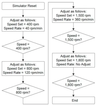
In Fig. 10, when one of the speed set button is commanded to be selected for speed increase on OIS (Operator Interface Station), the value goes to the controller via communication.
This makes the target value of the controller increase. As
a result, the positions of 6 IVs and 4 GVs go up according to their demands.
Because all the field instruments and drivers including valve positioners are ready for operation in this phase, all steam valves are being controlled by speed controller.
So, the speed control systems can know the positions of all steam valves including ESVs and RSVs, and can send the values to the dynamic model inside turbine simulator for calculation of turbine speed. Therefore, turbine speed can be increased or decreased in dynamic model with the actuators in the field moving and turbine not running. In this way, every condition of field instruments can be checked. Fig 12 tells the test procedure executed during stimulation test.
The simulation is to test and verify all of the speed control functions before actual speed up. This method of simulation test was performed according to the operation procedure after we install the speed control system in actual power plant.
B. Result
The test results of pre startup simulation are displayed here Fig. 13. When the operator resets the turbine on operator interface station, all of 6 ESVs and 6 RSVs go to their full open positions. When the operator selects a speed set and a speed rate, the 6 IVs go open to the 100% simultaneously at a predetermined rate, sequentially, the 6 GVs are governed by speed controller which causes the turbine speed to increase in dynamic model.
Fig. 13 shows that the position of IV20 fluctuates much at low speed but becomes small in proportional to the increase of speed. Fig. 13 shows also that the amount of IV20’s fluctuation becomes bigger and bigger when the speed rate is bigger. So, it is concluded that the speed error becomes bigger to the proportional to the speed rate.
Fig 10. Operator interface station.
Fig 11. Pre startup simulation.
Fig 12. Procedure of simulation. VII. ACTUAL OPERATION
Fig. 14 shows the resultant trends of actual operation of control system with no simulator running. The procedures of this operation are precisely the same with those of pre start up simulation. The quality of control in actual operation is better than that of the simulation because both the fluctuations of IV20 and GV5 in Fig. 14 (Actual Operation) are smaller than those in Fig. 13 (Pre Startup Simulation).
The IV20 does not oscillate and the position change of the GV5 is much smaller than that of simulation result. This means that we need to modify parameters in dynamic models such as frictional loss, windage loss, rotational inertia, valve stroking rate and admittance, etc. for more accurate simulation.
Also, the Fig. 14 shows that the IV20 fluctuates less than that of Fig. 13 and shows that the IV20 goes into stability faster than that of Fig. 13.
VIII. CONCLUSION
Dynamic and mathematical models of steam turbine and its components are developed by use of Stodola’s equation based on the physical law of energy conservation, mass conservation, momentum conservation and thermodynamic relations in this paper.
Comparison between the responses of the dynamic model with those of actual system is helpful to validate the degrees of precision of the developed model during start up.
The proposed dynamic model can be useful to control system design and V&V (Verification and validation) of control logic and to perform real-time simulations before startup in the field level.
Additionally, the decided parameters are very useful enough to operator education because the trends of important variables during pre-startup simulation and actual operation are not much different in their fluctuation. Moreover, the actual operation shows the better results than pre start simulation in detail.
REFERENCES
[1] Ali Chaibakhsh, Ali Ghaffari, “Simulation Modelling Practice and Theory,” 16 (2008) 1145.1162, 2008.
[2] M. Nagpal, A. Moshref, G.K. Morison, P. Kundur, “Experience with testing and modeling of gas turbines,” IEEE Power Engineering Society Winter Meeting, 2 (2001) 652.656, 2001.
[3] M. Wang, N.F. Thornhill, B. Huang, “Closed-loop identification with a quantizer,” Journal of Process Control 15 (2005) 729.740, 2005. [4] D. W. Kim, C. Youn, B.-H. Cho and G. Son, “Development of a power plant
simulation tool with GUI based on general purpose design software,” International Journal of Control, Automation, and Systems, vol. 3, no. 3, pp. 493-501, 2005.
[5] A. Stodola, Steam and Gas Turbine, vol. 1, Peter Smith, New York, 1945. Fig 14. Actual operation result.
Fig 13. Pre startup simulation result.
whether they are in its good state or not in this stimulation type method. For that purpose, dynamic models about steam turbine and its components are integrated into the hardware simulator.
On the basis of configuration shown in Fig. 11, all of the following function can be tested before actual operation.
- Turbine Arming and Speed Up
- Speed Control and Synchronization with Grid - Generator Load Up and Down
- Steam Valve Closure Test - Emergency Overspeed Trip Test - Load Dump Test on Normal Operation A. Method
In Fig. 10, when one of the speed set button is commanded to be selected for speed increase on OIS (Operator Interface Station), the value goes to the controller via communication.
This makes the target value of the controller increase. As
a result, the positions of 6 IVs and 4 GVs go up according to their demands.
Because all the field instruments and drivers including valve positioners are ready for operation in this phase, all steam valves are being controlled by speed controller.
So, the speed control systems can know the positions of all steam valves including ESVs and RSVs, and can send the values to the dynamic model inside turbine simulator for calculation of turbine speed. Therefore, turbine speed can be increased or decreased in dynamic model with the actuators in the field moving and turbine not running. In this way, every condition of field instruments can be checked. Fig 12 tells the test procedure executed during stimulation test.
The simulation is to test and verify all of the speed control functions before actual speed up. This method of simulation test was performed according to the operation procedure after we install the speed control system in actual power plant.
B. Result
The test results of pre startup simulation are displayed here Fig. 13. When the operator resets the turbine on operator interface station, all of 6 ESVs and 6 RSVs go to their full open positions. When the operator selects a speed set and a speed rate, the 6 IVs go open to the 100% simultaneously at a predetermined rate, sequentially, the 6 GVs are governed by speed controller which causes the turbine speed to increase in dynamic model.
Fig. 13 shows that the position of IV20 fluctuates much at low speed but becomes small in proportional to the increase of speed. Fig. 13 shows also that the amount of IV20’s fluctuation becomes bigger and bigger when the speed rate is bigger. So, it is concluded that the speed error becomes bigger to the proportional to the speed rate.
Fig 10. Operator interface station.
Fig 11. Pre startup simulation.
Fig 12. Procedure of simulation. VII. ACTUAL OPERATION
Fig. 14 shows the resultant trends of actual operation of control system with no simulator running. The procedures of this operation are precisely the same with those of pre start up simulation. The quality of control in actual operation is better than that of the simulation because both the fluctuations of IV20 and GV5 in Fig. 14 (Actual Operation) are smaller than those in Fig. 13 (Pre Startup Simulation).
The IV20 does not oscillate and the position change of the GV5 is much smaller than that of simulation result. This means that we need to modify parameters in dynamic models such as frictional loss, windage loss, rotational inertia, valve stroking rate and admittance, etc. for more accurate simulation.
Also, the Fig. 14 shows that the IV20 fluctuates less than that of Fig. 13 and shows that the IV20 goes into stability faster than that of Fig. 13.
VIII. CONCLUSION
Dynamic and mathematical models of steam turbine and its components are developed by use of Stodola’s equation based on the physical law of energy conservation, mass conservation, momentum conservation and thermodynamic relations in this paper.
Comparison between the responses of the dynamic model with those of actual system is helpful to validate the degrees of precision of the developed model during start up.
The proposed dynamic model can be useful to control system design and V&V (Verification and validation) of control logic and to perform real-time simulations before startup in the field level.
Additionally, the decided parameters are very useful enough to operator education because the trends of important variables during pre-startup simulation and actual operation are not much different in their fluctuation.
Moreover, the actual operation shows the better results than pre start simulation in detail.
REFERENCES
[1] Ali Chaibakhsh, Ali Ghaffari, “Simulation Modelling Practice and Theory,”
16 (2008) 1145.1162, 2008.
[2] M. Nagpal, A. Moshref, G.K. Morison, P. Kundur, “Experience with testing and modeling of gas turbines,” IEEE Power Engineering Society Winter Meeting, 2 (2001) 652.656, 2001.
[3] M. Wang, N.F. Thornhill, B. Huang, “Closed-loop identification with a quantizer,” Journal of Process Control 15 (2005) 729.740, 2005.
[4] D. W. Kim, C. Youn, B.-H. Cho and G. Son, “Development of a power plant simulation tool with GUI based on general purpose design software,”
International Journal of Control, Automation, and Systems, vol. 3, no. 3, pp. 493-501, 2005.
[5] A. Stodola, Steam and Gas Turbine, vol. 1, Peter Smith, New York, 1945.
Fig 14. Actual operation result.
Fig 13. Pre startup simulation result.