Simulated Annealing for Two-Agent Scheduling Problem with Exponential Job-Dependent Position-Based Learning Effects
Jin Young Choi*
작업별 위치기반 지수학습 효과를 갖는 2-에이전트 스케줄링 문제를 위한 시뮬레이티드 어닐링
최진영*
ABSTRACT
In this paper, we consider a two-agent single-machine scheduling problem with exponential job-dependent position-based learning effects. The objective is to minimize the total weighted completion time of one agent with the restriction that the makespan of the other agent cannot exceed an upper bound. First, we propose a branch-and- bound algorithm by developing some dominance /feasibility properties and a lower bound to find an optimal solution.
Second, we design an efficient simulated annealing (SA) algorithm to search a near optimal solution by considering six different SAs to generate initial solutions. We show the performance superiority of the suggested SA using a numerical experiment. Specifically, we verify that there is no significant difference in the performance of
between different considered SAs using the paired -test. Furthermore, we testify that random generation method is better than the others for agent , whereas the initial solution method for agent did not affect the performance of .
Key words : Two-Agent Scheduling, Exponential Learning Effect, Job-Dependent Position-Based Processing Time, Total Weighted Completion Time, Makespan, Branch-And-Bound Algorithm, Simulated Annealing
요 약
본 논문은 작업별 위치기반 지수학습 효과를 갖는 2-에이전트 단일기계 스케줄링 문제를 고려한다. 에이전트 는 가중 완료 시간의 합을 최소화하며, 에이전트 는 총소요시간에 대한 상한 값을 만족하는 조건을 갖는다. 본 연구에서는 먼저 우수 해/가능해에 대한 특성을 개발하고, 이를 이용하여 최적 해를 찾기 위한 분지한계 알고리즘을 설계한다. 또한 근사 최적 해를 구하기 위해 6가지 다른 초기해 생성 방법을 이용한 시뮬레이티드 어닐링 알고리즘을 제안한다. 수치 실험을 통해 제안된 알고 리즘의 우수한 성능을 검증한다. 실험 결과, 다른 초기해 생성 방법들 간에는 차이가 유의하게 발생하지 않았으며, 에이전트 의 작업 순서를 무작위로 생성할 때 성능이 좋아짐을 발견하였다. 반면에, 에이전트 의 초기해 생성 방법은 성능 에 영향을 미치지 않았다.
주요어 : 2-에이전트 스케줄링, 지수 학습효과, 작업별 위치기반 처리시간, 가중 완료 시간의 합, 총소요시간, 분지 한계 알고리즘, 시뮬레이티드 어닐링
Received: 28 August 2015, Revised: 8 December 2015, Accepted: 10 December 2015
*Corresponding Author: Jin Young Choi E-mail: [email protected]
An abridged version of this article was presented at the MISTA 2015 Conference (Choi, 2015).
1. Introduction
Two-agent single-machine scheduling problem can be found in various industrial applications where two agents compete for a single common machine to achieve their respective objectives. For example, we can consider a
production system under maintenance planning. The production department (agent) wants to operate the system without any idle time in order to maximize the system utilization. On the other hand, the maintenance department (agent) calls for frequent pauses of the production system in order to reduce the number of unexpected breakdowns of the system. Therefore, two departments (agents) share the production system, while pursuing different objective functions. Another example of the two-agent scheduling problems is the case of a classical problem in air traffic management for scheduling aircraft landings on a given set of runways. If two airlines (agents) have different performance measures such as safety and quality of service, each airline (agent) is definitely interested in maximizing the frequency cleaning/ checking the runways and minimizing the delay of the corresponding flights, respectively, in order to maximize the satisfaction of its own passengers (Agnetis, 2012).
This problem is a special case of general single-agent bi-criteria optimization model (Agnetis et al., 2004) because all jobs contribute to both objectives, and a key issue is to determine the non-dominated schedules for each objective in a sense that a better schedule for one objective makes the other objective worse. Furthermore, this problem has some characteristics as follows: (i) two objectives correspond to different two agents having their own jobs to process, (ii) they compete on the usage of a common processing resource, (iii) each agent has different performance measure, and (iv) only the jobs pertaining to one agent contribute to the computation of the objective function for itself.
Therefore, a typical methodology for simple single-agent bi-criteria optimization models such as using weighted objective functions of two agents cannot be applied, and the complexity of it is higher than that by simple single- agent bi-criteria scheduling problem (Agnetis et al., 2004), necessitating a new systematic approach.
Of particular interest is a two-agent single-machine scheduling problem with exponential job-dependent position- based learning effect. This means that each job has its own learning effect, implying that the learning in the production process of some jobs is faster than those of others.
Moreover, the actual processing time of a job is expressed as an exponential decreasing function of learning effect
and processing sequence. For example, performing similar tasks repeatedly can improve the skills of workers so that they can perform setups and handle raw materials faster, while reducing the actual processing time. This modeling concept is a plausible scenario in real-life manufacturing environment, deserving some attention.
However, to the best of our knowledge, in the literature there has been no research works on this specific issue considering two-agent, position-dependent, and job-dependent learning effect, simultaneously, whereas there were some works on simpler cases considering position-dependent processing times (learning/ aging) for two-agent or job- dependent learning effect for single agent as follows;
Since the concepts of the two-agent single-machine scheduling problem was first introduced by Baker and Smith (2003), many research works have been conducted on this topic, while learning/aging effect in a single-agent scheduling problem were firstly introduced by Biskup (1999) and Mosheiov (2001), respectively. Readers can find an extensive survey on scheduling problems with learning effects in Biskup (2008). Mosheiov (2005) showed that a V-shaped schedule is optimal for the problem of minimizing flowtime in a single-machine case. Kuo and Yang (2008) solved a single-machine scheduling problem with the cyclic process of an aging effect. Chang et al. (2009) worked on single- machine scheduling problems with a common due date under learning/aging effect consideration.
Meanwhile, two-agent scheduling problems with position- dependent processing times have received considerable attention in recent years, where actual processing times can be represented by using a linear function or an expo- nential function. Liu et al. (2010), Lee et al. (2010), Liu et al. (2011), and Wu et al. (2013) considered a linear function for computing actual processing times. On the other hand, Cheng et al. (2011), Wu et al. (2011b), and Li and Hsu (2012) applied an exponential function to represent actual processing times. All of these works took into account different performance objectives for two agents, which are functions of completion times such as (weighted) sum of tardiness, (weighted) sum of completion times, lateness, the number of tardy jobs, or upper bound of makespan, and so on.
Regarding the modeling concept of job-dependent learning
effect, it was suggested by Cheng and Wang (2000) for the first time. Mosheiov and Sidney (2003) studied a job- dependent learning curve where the learning of some jobs is faster than those of others. Then, Bachman and Janiak (2004) investigated a learning effect formulation on the single-machine case, and Wang and Xia (2005) extended it to multiple-machine case for a flow-shop consisting of an increasing series of dominating machines. However, they did not consider a two-agent case competing for a common resource.
Motivated by these remarks, in this paper, we inve- stigate a rather general problem, where two agents are included with an exponential position-based and job- dependent learning effect, while competing for a common single machine. In the context of the operational framework, we call it a two-agent single-machine scheduling problem with exponential job-dependent position-based learning effect. The objective is to minimize the total weighted completion time of one agent with the restriction that the makespan of the other agent cannot exceed an upper bound. We suggest some dominance and feasibility properties for a branch-and-bound algorithm (B&B), which can be used to find optimal solutions and to compare effectiveness of other algorithms considered. Furthermore, we design an efficient simulated annealing (SA) algorithm to search a near optimal solution and show its superiority of performance by using a numerical experiment.
The remainder of this paper is organized as follows. In the next section, we define the problem formally and suggest several dominance and feasibility properties related to the B&B algorithm. In Section 3, we design an efficient simulated annealing algorithm to obtain near-optimal solutions. The computational experiments are conducted in Section 4 and we conclude our discussion by suggesting some future works in Section 5.
2. Problem definition and a branch-and-bound algorithm 2.1 Problem definition
Two agent s and have set s of jobs
⋯ , ⋯ to process,
respectively, while competing for a single common machine.
The objective of agent is to minimize the total weighted completion time and agent wants to keep the makespan,
max , less than an upper bound . Each job for agent is assigned with a weight and a normal processing time
≤ ≤ . Each job for agent has a normal processing time ≤ ≤ . All jobs have job- dependent and position-based learning effect, so that actual processing time of job ∈ processed at the th position in a sequence, , can be expressed as an exponential decreasing function ∙
, where is a learning ratio of job ∈ . Then, using the three-field notation suggested by Graham et al. (1979), where is the number of machines,
denotes job characteristics, and describes objective functions, the scheduling problem under consideration can be represented as
max ≤
(1)
where is the completion time of job . Agnetis et al. (2004) showed that m ax ≤ is binary NP-hard. It implies that our problem in Eq. 1 is at least binary NP-hard, and we need an efficient solution approach to solve it. In our work, we suggest a B&B algorithm to obtain an optimal solution, and a simulated annealing algorithm for a near optimal solution.
2.2 Properties and a lower bound for a branch-and-bound algorithm
For a B&B approach, we first develop four dominance properties based on a pairwise interchange comparison method as follows. Suppose that we have two schedules
and s.t. ′ and ′, where is a scheduled part of jobs and ′ is a unscheduled part of jobs. Hence, jobs and
are in the th and th positions in , respectively.
can be obtained by interchanging two jobs and
in . By defining as the completion time of the last job in , we can compute the completion times of jobs and
as
Let us assume that we just sequenced after and are about to arrange , resulting in schedule . Then, we can derive certain conditions under which schedule is dominated by schedule . Specifically, we need two conditions for two agents such that (i) has smaller total weighted completion time for agent than that of , and (ii) the makespan of agent satisfies the upper bound condition. In addition, we need one more condition such that , implying that we can keep the dominance of over after arranging jobs in ′ in later steps. By defining , we have the following properties.
(Property 1) For ∈ ∈, if
≤
min
, then dominates .
Proof: Since ∈, the first condition is
≤
⇔
≤
Therefore, we have
≤ ⇔
≤ (2)
≤
⇔
≥
(3)
From , we have
⇔
(4)
Since there is no job for agent , we do not need the make- span condition for agent . From Eqs. 2-4, dominates , if
≤
min
.
Three further properties can be proved in a similar manner to Property 1.
(Property 2) For ∈ ∈, if
and ≤ , then dominates .
(Property 3) For ∈ ∈, if
and ≤ , then dominates .
(Property 4) ∈ ∈, if
≤
min
, then dominates .
Moreover, we have three more feasibility properties of a sequence as follows. Suppose that we have a sequence of jobs , where represents a sequence of jobs scheduled and is a set of jobs unscheduled. In addition, let and be the last th job scheduled and the completion time of it, respectively. Then, the following properties can be proved easily using the objective function requirement of agent .
(Property 5) If
with ∈ and ∩≠ ∅, then the sequence is non-promising.
(Property 6) If with ∈,
then the sequence is non-promising.
(Property 7) If ≤ ∩≠ ∅, and min ,
then the sequence is non-promising, where
min is the minimum actual processing time by any job in at the th position.
Based on these properties, we can apply a B&B algorithm to find an optimal solution (Hillier and Lieberman, 2015).
A node represents a partial or complete schedule and the initial node is empty, denoting none of jobs is scheduled.
Then, we can assign any job in the first position in a sequence and select a job for the second position, and so on. This is called a branching process. Hence, the basic idea is to branch a node into several nodes, each corresponding to scheduling one available job at that time point, and bound it by computing the potential minimum value of the total weighted completion time, called a lower bound, for agent , which can speed up the search procedure.
(Lemma 1) Suppose that there are jobs for agent
in so that their weights can be sorted in a non- increasing order, as ≥ ≥⋯≥ . Then, a lower bound of for a sequence corresponding to the state assigning only jobs in is
(5)
where , and and denote the weight and the completion time of the job scheduled in the
th order among jobs for agent in , respectively.
Furthermore, denotes the estimated minimum completion time of a job that can be scheduled in the th order among jobs for agent in .
Proof: The first term in Eq. 5 computes the sum of
weighted completion times of jobs for agent already scheduled. In the second term, without loss of generality, completion times, , are an increasing function of the processing sequence, and s' are decreasing function.
Therefore, is minimized (Hardy et al., 1967), providing a lower bound for .
For a given schedule , we suggest an efficient method to calculate in Eq. 5 as follows.
1. Identify the minimum actual processing times at the positions from th to th in , while allowing to select them from same jobs in .
2. Calculate completion times at those positions using the minimum actual processing times, denoted by
⋯ .
3. Assign jobs for agent to first positions and
jobs for agent to following positions.
4. If , adjust the sequence of
jobs to satisfy the upper bound condition for agent B as follows. Otherwise, go to (5).
(a) Check the upper bound condition of agent 's jobs from the th job in a backward manner.
(b) Whenever a job does not satisfy the upper bound condition, find one preceding last job for agent and interchange with it.
(c) Update as , where is the minimum actual processing time of the selected agent 's job for interchanging.
(d) Repeat (b) and (c) until we find first agent 's job satisfying the upper bound condition, or there is no more jobs to consider.
5. Stop with the minimum completion times of jobs for agent .
3. Design of SA using different initial solutions
As an efficient solution approach to find a near optimal solution, in this section, we suggest a simulated annealing (SA) algorithm, that was proposed by Kirkpatrick et al.
(1983). It is one of the most popular meta-heuristics used to solve combinatorial optimization problems based on trajectory search procedure. It starts from an initial trial solution and explores the solution space by taking steps in random direction, while accepting some deteriorating steps probabilistically. Therefore, it can escape from a local optimum and increase the possibility to find a better solution. As the algorithm proceeds, it focuses on the feasible region that might contain an optimal solution. The main features of the algorithm can be described as follows.
Objective function : During the search procedure, we evaluate a trial solution under consideration using the objective function for agent , which is to minimize the total weighted completion time of jobs for agent . We represent the objective function value for the current trial solution and next trial solution as and , respectively.
Initial solution : Since we need to generate a feasible initial solution and the upper bound condition for agent affects the feasibility of a solution under consideration, we first arrange the jobs for agent ahead in generating an initial solution, to make max as small as possible, following the jobs for agent . We can consider different methods to make the partial sequences for the two agents.
Specifically, we consider three methods to arrange jobs for agent such as (i) = random order, (ii) = shortest normal processing time (SPT) order, and (iii) = shortest weighted normal processing time (WSPT) order.
This is because the objective of agent is to minimize the total weighted completion time, and it might be achieved by arranging jobs based on the information of (weighted) normal processing times. In the case of scheduling jobs for agent , we suggest two methods to order jobs for agent
such as (i) = random order and (ii) = non-decreasing order of . Therefore, we can consider
× different methods to generate an initial solution.
Neighborhood generation : For a given trial solution, we select two jobs randomly and interchange them to generate next trial solution. After computing max of new sequence generated, we check the upper bound condition
for agent . If it is feasible, we call it next trial solution.
Otherwise, we reapply this procedure until we get a feasible one.
Move selection : Using the next trial solution, we compute the objective function and get . If , we accept it and update the current trial solution with it.
Otherwise, we can accept it with the acceptance probability defined as
(6)
where is a control parameter, called the temperature, which can change the tendency to accept a worse solution than the current one. If , the exponent part of Eq. 6 becomes negative, making in the range 0-1 as the probability. If it is rejected, then we repeat from the neighborhood generation step.
Temperature schedule : We notice that we can change the value of to control the acceptance probability. Since
becomes large as the value of is large, we can make the search of SA to perform in random direction by setting a large value of at the early stage, whereas we can focus on a special region by using small value of at the later stage of the algorithm. Based on this idea, we can design how to change the temperature, called the temperature schedule. First, we set the initial temperature using the initial objective function value as × . Then, after performing a fixed number of iterations at
, we decrease the value of by × , represented as × . We can repeat this procedure for a fixed number of steps , which is the number of times we change the temperature. Hence, the temperature schedule can be expressed as ×
⋯ .
Terminating condition : We terminate the algorithm after a fixed number of iterations defined as × .
4. A numerical experiment 4.1 Design of a numerical experiment
We designed a numerical experiment to evaluate the performance of the suggested B&B algorithm and six different , using different methods in the generation of the initial solution as follows.
First, we considered four different values of as
with . The value of was set by
minmax, where min and max are the minimum and maximum value of the makespan that can be made using all jobs for agent , respectively, and
is a real-valued parameter. We considered three different values of as . We computed the value of max as the sum of normal processing times of jobs for agent and min as the sum of minimum actual processing times at first positions in a sequence by allowing duplicated selection of jobs.
We performed a pre-testing of SA by generating some simple scheduling problems using and
. More precisely, for each configuration of
, we generated 30 problem instances using normal processing times and job weights randomly generated in the range , and learning effects randomly generated in the range . We solved problem instances using six SAs, and compared the performance of the SAs using
defined as
×
where is the total weighted completion time, and represents the SA using and as initial solution methods for agent and agent , respectively, as defined in Section 3. Using the pre-testing results, we set the parameter values of SA to × .
As a relative comparison method of the performance of different SAs, we defined the relative deviation percentage (RDP) of as
min
× .
We can calculate this performance measure by computing one RDP for each problem instance and compiling statistics such as mean, maximum, or standard deviation.
4.2 Experimental results
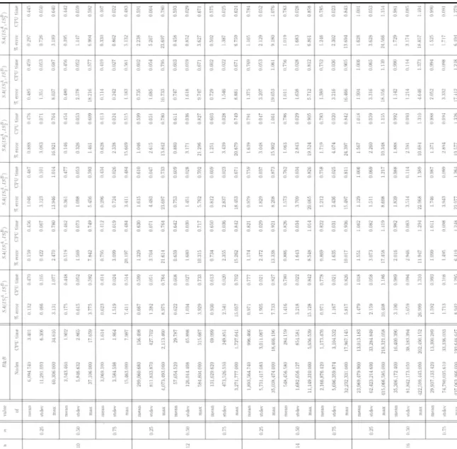
For each configuration of and the solution method, we generated 50 problem instances using the same parameter ranges and solved them using the B&B algorithm and six different SAs, . For each combination of and B&B (or ),
we calculated the mean, standard deviation (stdev), and maximum (max) number of generated nodes, CPU time (in seconds), and as in Table 1. Because small value of decreases the value of , it generates a tight upper bound for agent and makes B&B difficult to find an optimal solution, which were expressed as increasing values of node number and CPU time at , compared to other values of , for a fixed value of . The number of generated nodes and CPU time of B&B increased exponentially as increases. Specifically, B&B took a mean of 218,321.058 s (60.64 h) to find an optimal solution for the largest system .
The SAs showed good performance because they had low in almost all configurations of with a mean of less than 2%. The CPU time is within 1.1 s in all configurations, that is obviously favorable over that of B&B in environments requiring real-time scheduling. The CPU times were not affected by the size of problem instances because the CPU times were increased linearly as increases for a fixed value of . However, we could not see any linear relationship between the CPU times and the value of for a fixed value of . This can imply that the tightness of upper bound for agent does not affect the computation time of SA procedure.
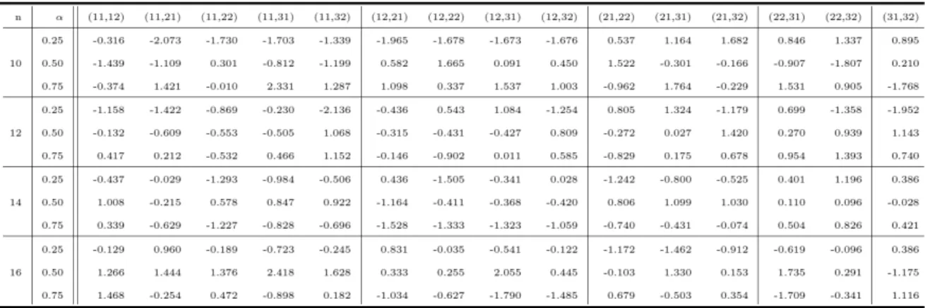
The performance difference of the proposed SAs in terms of was compared statistically by applying the paired -test. After denoting the difference of the th paired values of for two considered SAs, (for example, vs. ), as , we
Table 1. Results of numerical experiments (CPU time in s)
computed the sample mean difference and sample s t a n d a r d d e v i a t i o n , a s
a n d
. By the Central Limit Theorem (Hayter, 1996), has a normal distribution with unknown variance and hence, the test statistic defined as
(7)
has a -distribution with 49 degrees of freedom. Then, we can perform the -test by constructing the hypotheses set ≠ , where the hypothesis
≠ represents the tested assumption that the performance difference of the two considered SAs is significant. Table 2 displays the -values computed by Eq.
7 for the paired -test. The first row is the combination of indexes representing the initial solution generation methods as defined in Section 3. Hence, each of them denotes two