A Combined Approach of Pricing and (S-1, S) Inventory Policy in a Two-Echelon Supply Chain with Lost Sales Allowed

1. Introduction

Traditional inventory planning models for supply chains assume that all associated demand processes and revenue streams are exogenously determined. As a consequence, such models focus on operation cost minimization in the associated supply chains based on demand forecasts which are usually determined by marketing models. On the other hand, marketing models focus on determining pricing strategies and analyzing their impact on sales volumes and revenues, typically by rudimentary and simplistic treatment of operation cost in their supply chains(Chen, Federgruen

and Zheng, 2001). However, it has been noticed that simultaneous decision on pricing and inventory policy leads to more profit in a single-echelon inventory system(Kunreuther and Richard, 1971; Whitin, 1955).

Motivated by this notice, the combined approach of pricing and inventory policy has been intensively investigated for many single-echelon systems(Abad, 2001; Karlin and Carr, 1962; Pekelman, 1974). It has also been shown that the combined approach works better than any separated approach of treating the two problems individually. However, there are few studies about the combined approach for multi-echelon inventory systems. This provides the motivation for this paper to integrate the pricing and inventory

A Combined Approach of Pricing and (S-1, S) Inventory Policy in a Two-Echelon Supply Chain with Lost Sales Allowed

Chang Sup Sung^†․Sun Hoo Park

Department of Industrial Engineering, KAIST, Deajeon, 305-701

다단계

SCM

성창섭․박선후 한국과학기술원 산업공학과

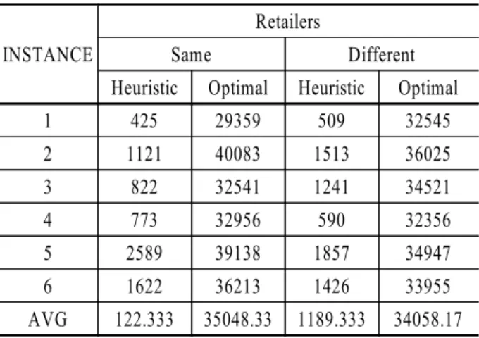
This paper considers a continuous-review two-echelon inventory control problem with one-to-one replenishment policy incorporated and with lost sales allowed where demand arrives in a stationary Poisson process. The problem is formulated using METRIC-approximation in a combined approach of pricing and (S-1, S) inventory policy, for which a heuristic solution algorithm is derived with respect to the corresponding one-warehouse multi-retailer supply chain. Specifically, decisions on retail pricing and warehouse inventory policies are made in integration to maximize total profit in the supply chain. The objective function of the model consists of sub-functions of revenue and cost (holding cost and penalty cost). To test the effectiveness and efficiency of the proposed algorithm, numerical experiments are performed with two cases. The first case deals with identical retailers and the second case deals with different retailers with different market sizes. The computational results show that the proposed algorithm is efficient and derives quite good decisions.

Keywords: inventory, pricing, two-echelon supply chain, lost sales, heuristic

This work was supported by Korea Research Foundation Grant (KRF-2002-041-D00557).

†Corresponding author : Chang Sup Sung, Department of Industrial Engineering, KAIST, Deajeon, 305-701, Fax : 042-869-3110, E-mail : [email protected]

Received April 2003; revision received February 2004; accepted May 2004.

control issues together in a two-echelon inventory system with stochastic demand processes incorporated.

The inventory system consists of a central warehouse and multiple retailers, where the warehouse distributes a single type of products to multiple retailers who will sell it to consumers. The retailers serve geographically dispersed and heterogeneous markets. Demands at each retail market arrive continuously but in a fashion of forming a non-linearly decreasing function of retail price in the market. The warehouse replenishes its inventory from an external supplier with ample capacity. Each retailer and the warehouse use the same (S-1, S) policy.

Generally, the (S-1, S) inventory policy is applied to situations where demand loss is not allowed or penalty changes are severe as in military service. Accordingly, the approach of combining the pricing issue and the issue of (S-1, S) inventory policy adaptation with lost sales allowed may be applied to dealing with expensive goods like jewelry or deluxe cars whose demand rates are subject to their price changes.

It has been reported in the literature that if the price and multi-echelon inventory decisions are made together at the same time, then the associated supply chain will get more profits due to increased sales and decreased operation cost, and so make the supply chain customers satisfied. Thereupon, this paper will focus on constructing a model that combines both the multi-echelon inventory decision and the pricing decision in the associated supply chain.

The exact cost for a single-echelon lost sales inventory system having Poisson-distributed demands and fixed leadtime has been derived in Hadley and Whitin (1963). Sung and Yang (1988) have considered (s, S) inventory policy with limited backlogging and stochastic leadtime. Smith (1997) has demonstrated how to evaluate and find the optimal (S-1, S) inventory policy for an inventory system with lost sales allowed but without any replenishment cost allowed and with generally distributed stochastic leadtime allowed. A METRIC-model has been suggested as one of the most widely known multi-echelon inventory models in Sherbrooke (1986).

Nahmias and Smith (1994) have considered a lost sales case for a multi-echelon system via the METRIC-model which has specifically considered periodic review batch order policies with partial lost sales allowed.

There are some marketing literatures studied on supply chain coordination between retailer and supplier which focuses on pricing. For example, Jeuland and Shugan (1983) have considered a simple pricing issue for a single-supplier and single-retailer system. Their model did not consider any inventory replenishment. The single-retailer part has been

extended to multi-retailer settings by Ingene and Parry (1995). Monahan (1984) has determined prices subject to the restriction that both supplier and retailer use identical order intervals. Lal and Staelin (1984) have considered a pricing problem with non-identical retailers, under the assumption that all demand processes are not exogenously given and inventory replenishment is made infrequently.

The approach of integrating inventory control and pricing issues together was first advocated by Whitin (1955). Both Whitin (1955) and Mills (1959) have addressed a single-period, single-location model to determine the associated single-price and supply quantity. Karlin and Carr (1962) have considered an in finite horizon model for a single item, under the assumption that a single price needs to be specified at the beginning of the planning horizon. Chen et al.

(2001) have considered both coordination (power-of- two) mechanism and non-coordination mechanism for multi-retailer systems under a periodic review inventory policy. Lee and Hong (2002) have integrated the pricing issue and the (r, Q) policy adaptation issue in a single-warehouse and single-retailer system with stochastic demand processes incorporated.

The organization of this paper is briefed as follows.

Section 2 presents the problem description and formulation. Section 3 analyzes the solution properties and proposes a solution algorithm based on the solution properties. Section 4 gives the computational results of some numerical examples, and Section 5 states conclusions.

2. Problem Description

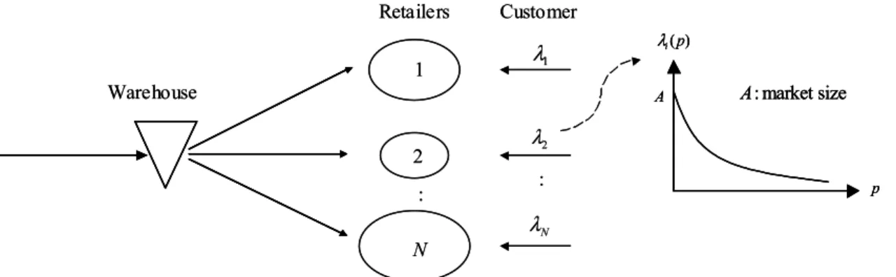
The proposed problem considers a two-echelon inventory system with single central warehouse and multiple retailers as depicted in <Figure 1>. The retailers, which have different market sizes, serve to satisfy customer demands and replenish the associated stocks from the central warehouse. The warehouse, in turn, replenishes its stock from an outside supplier.

The customer demand rate decreases exponentially as the price increases, while the retail price at each market is the same. The objective of the problem is to find the combined policy for inventory replenishment and pricing that maximizes long-run average profit in the associated two-echelon supply chain. There is a central planner who makes the pricing and inventory replenishment decisions. That is, the central planner makes both decisions simultaneously to maximize the total average profit of the two-echelon supply chain.

Demand process at each retailer follows a stationary Poisson process with constant arrival rate. When a

retailer is out of stock, any arriving demand at the retailer will be lost. However, when a stockout occurs at the warehouse, all demands from the retailers are fully backlogged and the backorders are filled according to a FIFO-policy. Each retailer and the warehouse use the same (S-1, S) policy.

The transportation time from the warehouse to any retailer is assumed to be constant. The transportation time from the external supplier to the warehouse is also constant. The external supplier is assumed to have infinite capacity, which means that the replenishment leadtime for the central warehouse is constant. The replenishment and backorder costs are assumed to be negligible, compared to the holding and stockout costs. Any units held in stock at the warehouse and the retailers incur holding costs per unit per time. A fixed shortage cost per lost customer is incurred at the retailers.

The objective of the problem is to maximize the long-run total average profit of the associated supply chain, which is defined as the difference between the associated total revenue and cost. The total revenue function can be easily defined by multiplying total sales by retail price. However, the cost function is more complex, so that some detailed analysis on the warehouse and the retailers should be made before deriving the associated cost function. The total cost consists of inventory holding costs at the warehouse and all the retailers, and penalty costs at all the retailers. Let us introduce the following notation:

N : Number of retailers

λi : Demand intensity at retailer _i, _i = 1,2,…,N λ₀ : Sum of customer demands arrived at the retailers ^=∑_{i = 1}^{N λi}

Λ : Demand intensity at the warehouse

L_i : Transportation time for delivery from the warehouse to retailer _i, _i = 1,2,…,N

L0 : Transportation time for delivery from the

external supplier to the warehouse

S0 : Order-up-to level at warehouse

Si : Order-up-to level at retailer _i, _i = 1,2,…,N

( S = S₁, S₂,...S_N )

h0 : Unit holding cost per unit time at the warehouse

hi : Unit holding cost per unit time at retailer _i, _i = 1,2,…,N

π_i : Unit penalty cost for lost sale at retailer _i, _i = 1,2,…,N

c : Unit purchasing cost at the warehouse

p : Unit retail price charged by retailer _i, _i = 1,2,…,_N

Ai: Market size of retailer _i, _i = 1,2,…,N α : Elastic coefficient of retail price _p

D_i : Costumer demand in the market served by retailer _i, _i = 1,2,…,_N =_Aie^-αp

G_i( ∙) : Sales revenue function at retailer _i, _i = 1,2,…,N

C0( ∙): Long-run cost function per unit time for the warehouse in steady state

Ci( ∙) : Long-run cost function per unit time for retailer _i in steady state, _i = 1,2,…,N

C^min_i ≡ min _siC_i(S_i, L_i) : minimum cost per unit time for retailer _i in steady state when the leadtime, L_i, is substituted for Li, _i = 1, 2,…,_N, given fixed _p

TC(∙): Long-run total cost function for the inventory system per time unit in steady state =^{C0( ∙) +∑}_{i = 0}^{N Ci( ∙)}

A queueing system analogy will be used when evaluating costs at the retailers, which has been adapted successfully in the analysis of inventory systems as in Sherbrooke (1986). It is noted that the demand process at the retailers follows a stationary Poisson process and the replenishment leadtime is

Figure 1. Two-echelon inventory system (1:1:N).

Customer Retailers

Warehouse

λ1

1

: 2

N

: market size A A

i( )p λ

p

λ2

λN

: Customer Retailers

Warehouse

λ1

1

: 2

N

: market size A A

i( )p λ

p : market size A A

i( )p λ

p

λ2

λN

:

stochastic, since orders from the retailers can be delayed at the central warehouse due to stochastic stockouts. According to Palm (1938), it is also noted that the steady state occupancy level is Poisson distributed with mean _λL, where _λ is the mean arrival rate and _L is the mean service time, which holds for i.i.d. service times. However, the stochastic leadtimes in the proposed problem are evidently not independent to each other. By the way, by disregarding any associated correlation, the number of outstanding orders will be approximated in this paper as to follow a Poisson distribution, as adapted in the METRIC- approximation in Sherbrooke (1986).

In the situation where lost sales are allowed, the corresponding queueing system of interest can be modeled as an M/G/S/S queue with _S servers, each with generally distributed service time and no queueing allowed. If the service times are independent random variables with mean _L , then the associated Erlang's loss formula can be viewed as stating the steady-state distribution of occupancy level at the retailer as

0

( ) / !

( ) 0

( ) / !

p j

s i

S p n

n i

A e L j

q j j S

A e L n

α α

−

−

=

= ≤ ≤

∑ ^{, where}

q^s(j) is the probability that _j servers (out of S) are occupied in steady state. Based on the METRIC approximation explained above, the number of outstanding orders at the retailer can be modeled as

q^s( j) .

Let the mean replenishment leadtime at retailer _i be Li and let q^s_i( j) be the steady-state probability of _j outstanding orders, given a desired-stock level Si. Then, the expected number of lost sales per unit time is derived as λ_{i i}q S^si( )_i =A e_i ^−αpq S_i^si( )_i and the expected number of units in stock is derived as

∑

Si

j= 0(Si- j)q^Siⁱ(j)= Si-[1-q^Siⁱ(Si)]Aie^{- αp}Li . The demand rate from retailer _i without loss allowed is derived as (1- q^Siⁱ(Si))Aie^{- αp}. Therefrom, the associated total cost function at retailer _i can be derived as

C S L p_i( , , )_{i i} = A e_i ^−αpπ_{i i}q S^Si( )_i +

+h Si( i− −[1 q S A ei^Si( )]i i ^−αpLi) ₍₁₎ In the backorder case, the demand process at the warehouse follows the same stationary Poisson process as at the retailers. However, in the lost sales case, the warehouse may not have the same Poisson process, because any demand from customers may be lost during leadtime intervals for the orders of the retailer placed to the warehouse. For example, if the

basestock level at a retailer is one, then the retailer leadtime will be included in the inter-arrival time interval between two successive demand arrivals at the warehouse from the retailer so that all the demands from customers arrived during the leadtime will be lost due to stockout at the retailer. Therefore, the associated demand process at the warehouse does not remain as the original Poisson process any longer. The remaining demand process will be rather complex to characterize.

Therefore, in this paper the demand process at the warehouse will be approximated as a stationary Poisson process but with adjusted arrival rate. The arrival rate is assumed to be _Λ where _Λ depends on how much demand is lost at all the retailers, which is determined as

1

(1 ⁱ( ))

N p S

i i i

i

A e^−α q S

=

Λ =

∑

Now, given a fixed deterministic leadtime L0, we can find the average holding cost incurred at the warehouse as a function of _Λ and S₀.

0

0

0 0 0 0 0

0

( )

( , ) ( ) exp( )

!

S j

j

C S h S j L L

= j

Λ =

∑

where _Λ is the function of Si and _p, so that Eq. (2) can be incorporated as

0 0

1

0 0 0 0

0

( (1 ( )) )

( , , ) ( )

!

i

N p S j

S i i i

i j

A e q S L

C S S p h S j

j

−α

=

=

−

= − ∑

ur ∑

0 1

exp( ^N _i ^p(1 _i^Si( )) )_i

i

A e^−α q S L

=

−∑ − ⁽⁴⁾

The mean delivery delay can also be derived in consideration of stockout at the warehouse by using

B0, the average number of backorders at the warehouse, which can be calculated as

0

0

0 0 0

1

( )

( ) exp( )

!

j

j S

B j S L L

j

∞

= +

=

∑

Then, the Little’s formula is applied to obtain the average delivery delay, B0/Λ . Therewith, the mean leadtime for retailer _i is derived as

0/

i i

L = +L B Λ ⁽⁶⁾

The total revenue function can be represented as ( , ) ^p(1 ^Si( ))( )

i i i i i

G S p =A e^−α −q S p c− ⁽⁷⁾

The total cost function is obtained in the associated supply chain as

0 0

1

( ) ( , , ) ^N i( , , )i i i

TC C S S p C S L p

=

⋅ = ^ur +

∑

As mentioned above, a central planner makes the pricing and inventory replenishment decisions together so as to maximize the long-run average profit in the two-echelon supply chain, which is equal to the total revenue minus cost, expressed as

⁰ 1

( , , ) ^N _i( , )_i

i

TP S S p G S p

=

=

∑

ur

(9) ^{0 0} 1

( , , ) ^N i( , , )i i i

C S S p C S L p

=

 

− ^ur +

∑

It can be represented as the function of S0, Si, and

p which is given as

0

1

( , , ) ^N _i ^p(1 _i^Si( ))(_i )

i

TP S S p A e^−α q S p c

=

=

∑

ur

0 0

1

0 0

0

( (1 ( )) )

( )

!

i

N p S j

S i i i

i j

A e q S L

h S j

j

α

−

=

=

−

− −

∑

∑

^exp( ₁ ^{(1 i( )) )0}

N p S

i i i

i

A e^−α q S L

=

−

∑

1

( ) ( [1 ( )] )

i i

N p S S p

i i i i i i i i i i

i

A e^−α πq S h S q S A e^−α L

=

−

∑

3. Solution Procedure

The objective of the proposed problem is to find the optimal inventory positions S^*0 and and _S ^* the optimal price _p^* together which maximize the total supply chain profit. The total profit is calculated by subtracting the total cost at the warehouse and all the retailers from the total revenue of the retailers.

Inventory holding costs at the warehouse and all the retailers and penalty costs at all the retailers for lost sales cases are considered. To maximize the total profit, the total revenue must be maximized, while the total cost is minimized. As shown in Eq. (10), the total profit function is non-linear so that each involved decision variable is hard to clearly find its mathema- tical feature. Therefore, the near-optimal solution will be found by using a heuristic search algorithm. For the search, several solution properties will be characteri- zed in this chapter.

Lemma 1

( , , )i , .

i i i i

C S L p is convex with S given fixed L and p Proof. ^{C S L pi( , , )i i} can be proved to be convex in _Si with _Li fixed, referring to Smith (1997), and the value of _p is not subject to _Si’s. This implies that

( , , )i

i i

C S L p is convex too, given fixed _p . This completes the proof.

Given _Li and _p, the optimal order-up-to-level _Si, which minimizes the cost of the retailers, is obtained by a local search procedure. _Li is a function of _Λ and S0 as shown in Eqs. (5) and (6). This implies that the optimal order-up-to-level _Si can be found based on Lemma 1. The retail price _p and order-up-to-level at the warehouse _S0 are decision variables and _Λ is a value calculated from Eq. (2). For the given random variable _Λ, _Si is calculated, with which _Λ is updated as in Eq. (2). Therewith, given _p and _S0, the optimal value of _Si can be calculated.

Lemma 2

, min ( , ) min ( , )

i i

s i i i s i i i

Given p fixed C S L ≤ C S L Proof. Let Ci^min be the minimum cost per unit time for retailer _i in steady state when the leadtime, _Li, is substituted for _Li, _i = 1,2,…,_N, given fixed _p. It is represented as ^minsiC S Li^{( , )}i i . Then, it is needed to show that ^minsi C S Li^{( , ) min}i i ≤ siC S Li^{( , )}i i for Li ≤Li . Let _li be an arbitrarily chosen leadtime, where

i i i

L ≤ ≤l L . Consider the cost C S l , where _i( , )_{i i} Si is set at its optimal value for each _li . Start with li=Li

and let _li be continuously lowered until it reaches the level _Li as ^{li =Li}. Since ^{C S li( , )i i} is a continuous function of _li , for fixed _Si , it is also a continuous function of _li. Moreover, the fact that _Si minimizes the costC S l_i( , )_{i i} implies the relation C S li^{( , )}i i ≤C Si⁽ i

1, )l_i

− . For notational simplicity, the index _i will be omitted from all the variables. Thereupon, let

Ae ^αp

λ= ⁻ .

It can then be shown that ( , )

(1 ^s( )) ( )( (^s 1)

C S l

h q S h l q S

l λ λ λ πλ

∂ = − − + + −

∂

−q S^s( )+q S^s( ) ).² ①

Moreover, the relation ( , )C S l ≤C S( −1, )l implies that

1( 1) ( ).

s s

h q S q S

h lλ +λπ ^{≤ − − −} ②

Let ^{Κ =}_{λ λ πλ(h l}¹_{+ )} ^{∂C S l( , )}_∂l ^. From Eq. ①, it holds that

( ( ) 1)^{s s}( 1) ^s( ) ^s( ) .2

h q S q S q S q S

h lλ πλ

Κ = − + − − +

+

Multiplying the right-hand side of Eq. ② by _K g i v e s (recalling that ^{q Ss( ) 1<} )

Κ ≥⁽q^s−1(S− −¹⁾ q S^s( ))( ( ) 1)q S^s − +q S^s( −1) −q S^s( )+q S^s( )²

1 1

1 1

( 1) ( ) ( 1) ( 1)

( 1) ( ) ( ( 1) ( ))

0.

s s s s

s s s s

q S q S q S q S

q S q S q S q S

− −

− −

= − − − + −

= − − −

= ③

(Detail expression of ③)

From the definition of q Ss( −1), we have

( 1) ( ) S

s s

q S q S

λL

 

− =  . It can be shown following equation:

1 ( ) ( )

1( 1) ( 1) ,

! !

0 0

( ) 1 ( 1)!

( 1) .

( ) 0 ! 1 ( )

! , 0

( )

1( 1) ( 1)

!

n n

s L s L

s s

q s q s

n n

n n

L s s s

where q s

s L n n n

s L n Let U

n n

L s

s s

q s U q s U

S

λ λ

λ λ λ

λ

 −   

   

− −  ∑ = −  ∑ 

 =   = 

   

−

− = −

∑=

= ∑−

=

 

 

− − = −  + 

 

 

( ) 1

1( 1) ( 1) ( 1)

!

( ) 1

( 1) ( 1)

! ( ) 1( 1)

L s

s s s

q s q s q s

S U

s L s

q s q s

S s s q s q s

λ λ

− − − − = −

= − − −

= − −

Then we have ^qs−1(s− −^{1) q ss(} − =^{1) q s qs( ) s−1} (s−1).

Consequently, _{K ≥ 0}, so that C S L is a _i( , )_{i i} non-decreasing function for Li ≤Lⁱ. Let S L( )_i =

arg min_siC S L_i( , )_{i i} . Then, the relation ( ( ), )C S L L_{i i i} ≤ ( ( ), )

i i i

C S L L holds. Let ( ) arg minS L_i = _siC S L_i( , )_{i i} . Then, the relation ( ( ), )C S L L_{i i i} ≤C S L L_i( ( ), )_{i i} holds.

Therefore, the relation min ( , ) min

i i

s C S Li i i ≤ s

( , )i

i i

C S L for Li≤Li holds.

This completes the proof.

Lemma 3

0 0 0 0 0 0

, ( , ) ( , )

Given p fixed C S λ ≤C S Λ holds with S Proof. _λ0 is the sum of customer demands arrived at all the retailers, so that ^{Λ ≤λ0}. Then, it is only needed to show that ^{∂C S0( , )}_∂Λ^{o Λ ≤0}, which is shown as

0

0 0 0

( , )

exp( )

C So

h L L

∂ Λ = − −Λ

∂Λ

0 1

0 0

0 0

1

( ) ( )

( )

! ( 1)!

S j j

j

L L

S S j

j j

−

=

 + −  Λ − Λ 

  − 



∑

0 1 0

0 0

0

( )

exp( )

! 0.

S j

j

hL L L

j

−

=

= − −Λ Λ

≤

∑

This completes the proof.

Theorem 1

, _lb( )0

Given p fixed TC S is a lower bound for ,

the cost function

min

0 0 0 0

0

( ) ( , ) ^N .

lb i

i

TC S C S λ C

=

≡ +

∑

Proof. Axsater (1993) has proved the convexity of

0( , )0 0

C S λ in _S0. By Lemma 1, 2, and 3, given _p fixed, it is found that TC S is a lower bound for _lb( )0

the cost function ^{( 0) 0( 0, 0)} ₀ ^{m in}

N

lb i

i

TC S C S λ C

=

= +∑ _.

Moreover, the cost function TC S_lb( )0 is convex in _S0. This completes the proof.