Modeling and $H_{\infty}$ Optimal Control Design for a Hydraulic Unit in ESP

(1)

Modeling and H

∞

Optimal Control Design for a Hydraulic Unit in ESP

Seung-Han You

^†

, Jin-Oh Hahn

^*

, Young Man Cho

^**

and Kyo Il Lee

^**

ESP 유압 유니트의 모델링 및 H_∞ 최적제어

유승한^† · 한진오^* · 조영만^** · 이교일^**

Key Words : Direct yaw moment control(요 모멘트 제어), Hydraulic unit(유압 유니트), System iden- tification(시스템 식별), H_∞ optimization(H_∞ 최적화)

Abstract

This paper deals with feedback control of a hydraulic unit for direct yaw moment control, a method used to actively maintain the dynamic stability of an automobile. The uncertain parameters and complex structure naturally call for empirical modeling of the hydraulic unit, which readily results in a control-oriented model with high fidelity. The identified model is cross-validated against experimental data under various conditions, which helps to establish model uncertainty. Then, the H∞ optimization technique is employed to synthesize a controller with guaranteed robust stability and performance against the model uncertainty. The performance of the synthesized controller is verified using experimental results, which shows the viability of the proposed approach in a real-world application.

1. Introduction

The current automotive industry must cope with ever-stringent demand for the driver assistance systems since such capabilities of a vehicle as preventing fatal accidents and protecting passengers are increasingly recognized in the market as a necessity rather than a luxury. To reflect on such a trend, extensive research has been carried out on a variety of driver-subsidiary, active vehicle control methods to hold vehicles back from unstable operation. The following approaches summarize such efforts: steering intervention by differential brakes, vehicle dynamics control (VDC), vehicle stability control (VSC), vehicle stability assist (VSA) as well as direct yaw moment control (DYC) (Pilutti et al., 1999; Van Zanten et al., 1998; Tseng et al., 1999; Yasui et al., 1996; Nishimaki et al., 1999).

ESP that is the topic of this paper maintains rota- tional vehicle stability by generating compensatory arti-

ficial yaw moment through application of different brake forces to the individual wheels. In this respect, the hydraulic unit in an ESP is responsible for brake pressure control and thereby plays a key role in the directional stability of an automobile. Consequently, the hydraulic unit in an ESP must be precisely controlled to reliably supervise the yaw stability. Despite its practical significance, however, the lower level control of the hydraulic unit in an ESP has not fully addressed yet compared to its upper level counterpart for the overall vehicle dynamics (e.g., Van Zanten et al., 1996).

This paper presents a robust control of hydraulic unit for ESP, which begins with building a control-oriented mathematical model. Its multiple unknown parameters and complex structure does not allow in a straightfor- ward manner the physical modeling of the hydraulic unit in an ESP. Instead, an empirical modeling approach (Ljung, 1999) is taken in this paper to yield a black-box model that captures prominent dynamics of the hydraulic unit essential to control design. By meticulously ex- amining the fidelity of the empirical model under various conditions, a control-oriented model is established with corresponding uncertainty. Then the H∞ optimization technique (Skogestad & Postlethwaite, 1996; Doyle et al., 1992; Zhou & Doyle, 1998) is employed to syn-

† 회원, 서울대학교 대학원 기계항공공학부 E-mail : [email protected]

TEL : (02)880-7143 FAX : (02)883-1513

* ^회원, 공군사관학교 기계공학과

**

(2)

thesize a feedback controller with guaranteed robust stability and performance. The effectiveness of the proposed controller is experimentally verified to show its viability in real-world application.

2. Modeling of Hydraulic Unit for ESP

Operation principles and modeling aspects of the hydraulic unit in an ESP are detailed in Hahn et al. (2003), which finally yields the following empirical model:

( )

u

( )

s

s s

y 100

78 . 31

03 . 32 555 . 0

+ +

= − (1)

where y

( )

s is the wheel brake pressure and u

( )

s is the effective brake pressure variation at the wheel in the steady state.

3. H

∞

Optimal Control Design

3.1 Motivations for H∞ Control

It is well known that the utmost goal of feedback control is to minimize the sensitivity of the overall closed-loop system. From this perspective, a feedback controller for the ESP hydraulic unit is required to pos- sess sufficient level of robustness to model parametric uncertainty (which is the most salient source of disturbance exerting an adverse effect on the performance of the controller) due to the following reasons. First, the identified model of the hydraulic unit in the previous section may fail to guarantee its fidelity beyond the frequency range considered in the system identification procedure. Furthermore, the identified parameters of the ARX model (1) are susceptible to change with respect to such operating conditions as oil temperature. Be- tween robust and adaptive alternatives available for control to grant robustness to control system, however, adaptive approaches to the control of the ESP hydraulic unit are not so appealing since the pressure command signal usually suffers from lack of richness. In addition, the non-minimum phase nature of the identified model makes it extremely demanding to apply standard nonlinear control algorithms (Kahlil, 1996; Slotine & Li, 1991) such as input-output feedback linearization and Lyapunov re-design (internal dynamics becomes unstable). Therefore, robust control via H∞ optimization can be an attractive candidate to solve the control problem considered in this paper.

3.2 H∞ Control Synthesis

A schematic diagram for robust feedback control of the ESP hydraulic unit is shown in Fig. 1, where r

( )

s is the commanded wheel brake pressure signal, y

( )

s is the measured wheel brake pressure signal, v

( )

s is the

tracking error, u

( )

s is the control input signal and

( )

s

w is the model uncertainty. Besides, z₁

( )

s and

( )

s

z₂ are frequency-shaped error and plant output signals, respectively. K

( )

s denotes the feedback controller to be synthesized in this section, and G

( )

s is the plant model (1). The filters W₁

( )

s and W₂

( )

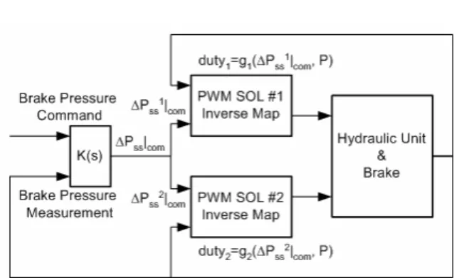
s are frequency shaping functions (or frequency weights) used to mathematically describe the performance and robustness specifications, respectively. It is noted that the plant uncertainty is modeled by output multiplicative uncertainty (Skogestad & Postlethwaite, 1996; Doyle et al., 1992; Zhou & Doyle, 1998) as shown in Fig. 1.

Extensive test results on the laboratory experimental set-up (Hahn et al., 2003) indicate that the steady state responses of the solenoid valves are highly repetitive except for duty ratio signals that are very small in magnitude, and the controller design procedure neglects the existence of the nonlinear steady state maps for SOL1 and SOL2 based on the postulation that the input disturbance induced by the variations in the steady state performance maps of SOL1 and SOL2 is not so significant in deteriorating the closed-loop performance compared to the output disturbance caused by the parametric uncertainty of the dynamic portion of the hydraulic unit model G

( )

s . Therefore, the controller output u

( )

s is assumed to be the corrective pressure variation signal to drive the pressure tracking error to zero during the controller design procedure. Instead, the pressure variation signal calculated by the controller K

( )

s is con- verted to the equivalent duty ratio signals before it is fed back to the hydraulic unit as shown in Fig. 2.

Fig. 1 The ESP hydraulic unit control problem

Fig. 2 Implementation of control system

(3)

In Fig. 1, the sensitivity and complementary sensitivity functions are defined as follows:

( ) ( )

≡

( )

=[1+G

( ) ( )

sK s

(

1+W₂

( ) ( )

s∆s

)

]⁻¹

s r

s s e

S_p (2a)

( ) ( )

( )

S

( )

s s

r s s y

T_p ≡ =1− _p (2b)

where ∆

( )

s is an arbitrary stable complex function with ∆

( )

jω <1 for ∀ . The subscript ‘p’ implies ω that the transfer functions are perturbed ones. It is not strenuous to derive the following robust performance condition for the problem setting in Fig. 1 (Doyle et al., 1992; Zhou & Doyle, 1998):

2 1

1 + <

T ∞

W S

W (3)

where S

( )

s and T

( )

s are nominal sensitivity and complementary sensitivity functions defined as follows:

( )

s =[1+G

( ) ( )

sK s]⁻¹

S _(4a)

( )

s =G

( ) ( )

sK s[1+G

( ) ( )

sK s]⁻¹

T _(4b)

The inequality in (3) can be re-stated in H∞ optimization language as follows:

( )

∞  ∞



 



≡ 

T W

S K W

K

K 2

min 1

min N (5)

The corresponding generalized plant (Balas et al., 2001;

Gahinet et al., 1995) P can be derived using the defi- nition of linear fractional transformation (LFT) (Sko- gestad & Postlethwaite, 1996; Zhou & Doyle, 1998):



 



=

22 21

12 11

P P

P

P P (6a)

( )

_



 



=

≡ WT

S K W F_l

2

, 1

P

N (6b)

with u

( )

s =K

( ) ( )

svs , where F is the lower LFT. The _l generalized plant is then found in the following form, based on which H∞ optimization may be carried out:



 





















−

=



 



= 

















u r G

G W

G W W

u r v z z

1

0 ₂

1 1

2 1

P (7)

The generalized plant (7) is shown in Fig. 3.

Specifying the performance and robustness requirements is a crucial stage in the H∞ controller design. In particular, it is essential to accurately define the amount of uncertainty inherent in the plant model, since the performance specification is closely related to the uncertainty; in other words, at every frequency point of interest, trade-off between performance and robustness is required to render the control design problem a solvable one. This paper first experimentally identifies the amount of plant parametric uncertainty and then seeks to design a controller that maximally achieves the desired closed-loop characteristics.

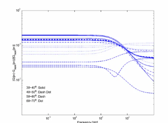
In the hydraulic unit considered in this paper, the most salient source of the model uncertainty stems out from the variation of oil characteristics such as bulk modulus with respect to the operating condition of the hydraulic unit such as oil temperature and pressure level at the brake chamber. Specifically, it may signifi- cantly alter the dynamic response characteristics of the solenoid valves as well as the hydraulic pipelines. To assess the amount of model uncertainty with respect to the oil temperature, 16 ARX models of the hydraulic unit are identified within the oil temperature range of interest (30~70[°C] in this paper), and their percentage variations with respect to the control design model are evaluated as follows:

( ) ( ) ( )

( )

^ω ^ω

ω ω

j G

j G j j G

G

nom

− nom

=

∆ (8)

where G_nom

( )

j^ω is the nominal transfer function and

( )

jω

G is its perturbed counterpart. As shown in Fig. 4, the 16 ARX models exhibit an upper bound of approximately 20[%] magnitude of the output multiplicative uncertainty up to 10[Hz]. However, the assessment in Fig. 4 is effective only within the identification frequency of 15[Hz], since the model may fail to preserve its fidelity beyond this frequency envelop. Accordingly, this paper assumes that the amount of uncertainty in- creases from 20[%] at low frequency ranges to 100[%]

at the identification frequency, reaching 200[%] at high frequencies, which can be described by the following frequency shaping function W₂

( )

s :

( )

2 90 2 . 0 90

2 2

2 2 2

+

×

= + +

≡ +

s s M

s A s s

W

ω

ω (9)

It is noted that the amount of uncertainty of 200[%] at high frequency region is arbitrarily chosen but can be adjusted without violating the robust performance criterion stated in (3); recall that the region of severest performance-robustness trade-off is the crossover region and not the low frequency (where sensitivity function is small) and high frequency (where complementary sen-

(4)

Fig. 4 Uncertainty imposed by oil temperature variation

Fig. 5 Sensitivity / complementary sensitivity functions

Given the amount of uncertainty to be considered in the control design process, the frequency shaping function for the performance specification is selected for the closed-loop system to achieve the desired closed-loop characteristics as much as possible, in the presence of the model uncertainty as well as the right-half-plane zero included in the hydraulic unit dynamics. Especially, the performance requirements on the hydraulic unit in this paper are 1) to keep the steady state brake pressure tracking error as small as possible, and 2) to maximize the speed of brake pressure response, i.e. the bandwidth of the closed-loop system. It is well known that the ma- jor constraint in defining the performance specification is the waterbed effect represented by the Bode sensitivity integral (Skogestad & Postlethwaite, 1996). Firstly, the non-minimum phase zero z_RHP of the hydraulic unit dynamics at approximately 9[Hz] acts as an obsta- cle to the achievable closed-loop bandwidth by impos- ing the following restriction on the frequency shaping function W₁

( )

s according to the maximum modulus theorem (Skogestad & Postlethwaite, 1996; Doyle et al., 1992; Zhou & Doyle, 1998):

( )

1

1 z_RHP <

W (10)

To emphasize the tracking with small steady state error, the DC value of 10⁵ is assigned to W₁

( )

s , which is equivalent to 10^-3[%] steady state error. Other parameters of W₁

( )

s in (11) are selected so that the sensitivity function is shaped with possibly maximal gain crossover frequency as well as guarantees the robust performance criterion (3):

( )

₅

1 1

1 1 1

10 9 3 9

× −

+ + + =

+

= s

s A

s M

s s

W ω

ω

(11)

It is noted that simple first order filters are used to define the frequency shaping functions to keep the order of controller as small as possible, since the order of the H∞ controller is equal to that of the generalized plant (Zhou & Doyle, 1998).

Fig. 5 shows the sensitivity and complementary sensitivity functions obtained using the designed H∞ controller, along with the frequency shaping functions. The gain and phase margins of the resulting loop gain are 3.28[db] and 66.2[°], respectively, and the maximum H∞ norm of N

( )

K is 0.98, which means the robust performance objective is satisfied.

4. Experimental Results

The performance of the designed H∞ controller is ex- amined over a variety of oil temperature conditions. A 3^rd order version of the originally 4^th order H∞ controller is obtained using the balanced truncation technique (Skogestad & Postlethwaite, 1996) and implemented on the real-time laboratory experimental set-up.

Experiments are first conducted at the oil temperature region where the model for the hydraulic unit is identified (about 50[°C]). Fig. 6 (a) shows the responses of the controlled hydraulic unit to step pressure increase from initial wheel brake pressure of 5[bar] (the hydraulic unit is expected to experience this type of command when it is activated), and those to step pressure de- crease to final wheel brake pressure of 5[bar] is given in Fig. 7 (a) (the hydraulic unit is expected to experience this type of command when it is deactivated). It can be seen that the steady state pressure tracking errors are close to zero in line with the design specification. In addition, all of the controlled responses shown in Fig. 6 exhibit the transients with duration less than 0.3[sec]

regardless of the magnitude of step reference command, which, together with the steady state accuracy, appears to be superb enough for real-world application.

To investigate the performance of the H∞ controller at intermediate pressure ranges, responses of the hydraulic unit to step pressure commands from different pressure levels to final wheel brake pressure of 50[bar] are pre-

(5)

sented in Fig. 8. The oil temperature is also approximately 50[°C] for this experiment. The results also exhibit consistent trends with those in Fig. 6 and Fig. 7, i.e.

negligible steady state tracking errors and fast transient characteristics.

Fig. 6 Step response from 5[bar] to higher pressures

Fig. 7 Step response from higher pressures to 5[bar]

Fig. 8 Step response from lower pressures to 50[bar]

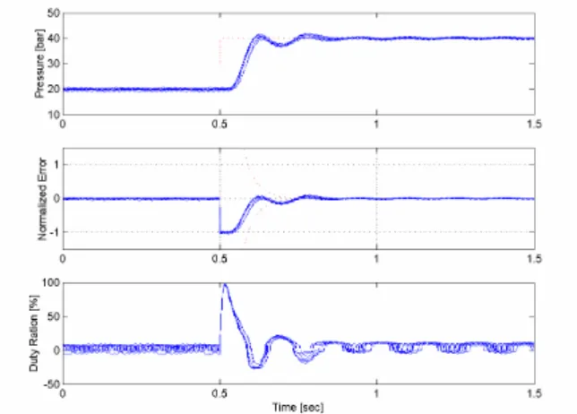
Finally, the controlled responses of the hydraulic unit to step pressure command at different oil temperatures are shown in Fig. 9 to validate the robustness of the H∞

controller to parametric variations of the identified

model, where seven identical responses within the oil temperature span of 30~70[°C] are shown together. It can be seen that the trajectories of the responses of the hydraulic unit are very similar to one another regardless of the oil temperature variations, which verifies that the performance of the H∞ controller is highly reliable over the oil temperature envelope of interest. To quantita- tively evaluate the closed-loop performance and ascer- tain whether the performance requirement described by the frequency weight W₁

( )

s is satisfied, the corresponding normalized tracking errors are shown in Fig. 9, respectively, together with the upper bound of the error trajectory specified by W₁

( )

s . It is noted that the sensitivity function S

( )

s is the transfer function from the command r

( )

s to the error e

( )

s , and its upper bound

( )

s W₁

1 provides the error response with worst quality, i.e. slowest decay rate with largest steady state error.

The upper bound ρ

( )

s of the error signal is obtained in terms of the step response of W₁

( )

s :

( ) ( )

s

R s

s s

R s s W

1

1 9 10 5

3 9 1

−

− 











× +

+

=

ρ = (12)

where R is the magnitude of the step command signal.

The results shown in Fig. 9 indicate that the performance requirements are indeed mostly satisfied except at the region of transition from transient to steady state, which appear to be due to such factors not explicitly considered in the control design process as local uncer- tainties in the steady state performance maps for SOL1 and SOL2 (especially those for small-in-magnitude duty ratio signals), saturation of control effort experi- enced by SOL1 and SOL2, and the discrete-time implementation of the controller designed in the continu- ous-time domain (digitization, quantization, and so on).

Fig. 9 Step responses at different oil temperatures

(6)

It is noted that the transients of the responses to the commands close to the pressure limit of the hydraulic pump (which is 60[bar] for the experimental set-up in this paper) appear more sluggish than those to lower command levels. However, this may not be a significant problem in actual vehicle, since it can be avoided by increasing the pressure limit whenever necessary with appropriate control of the hydraulic pump.

5. Conclusions

An H∞ optimization-based feedback approach to the control of a hydraulic unit in an ESP is presented in this paper. A simple model of the hydraulic unit with high fidelity is developed using experimentally estimated steady state performances of the solenoid valves and the ARX-model-based system identification technique. A robust controller that meets the robust stability and performance requirements against the model parametric variations is synthesized using the H∞ optimization technique. Experimental results indicate that the proposed approach can readily find a room for application on real-world automotive safety problems.

References

(1) Pilutti, T., Ulsoy, G., & Hrovat, D., 1998, “Vehicle Steering Intervention through Differential Braking,”

ASME J. Dynamic Systems, Measurement and Control, 120, 314-321.

(2) Van Zanten, A.T., Erhardt, R., Landesfeind, K., &

Pfaff, G.., 1998, “VDC Systems Development and Per- spective,” SAE 980235.

(3) Tseng, H.E., Ashrafi, B., Madau, D., Brown, T.A., &

Recker, D., 1999, “The Development of Vehicle Stabil- ity Control at Ford,” IEEE/ASME Trans. Mechatronics, 4, 223-234.

(4) Yasui, Y., Tozu, K., Hattori, N., & Sugisawa, M., 1996, “Improvement of Vehicle Directional Stability for Transient Steering Maneuvers Using Active Brake Control,” SAE 960485.

(5) Nishimaki, T., Yuhara, N., Shibahata, Y., & Kuriki, N., 1999, “Two-Degree-of-Freedom Hydraulic Pres- sure Controller Design for Direct Yaw Moment Con- trol System,” JSAE Review, 20, 517-522.

(6) Van Zanten, A.T., Erhardt, R., Pfaff, G., Kost, F., Hartmann, U., & Ehret, T., 1996, “Control Aspects of the Bosch-VDC,” Proc. International Symposium on Advanced Vehicle Control, 573-608.

(7) Ljung, J., 1999, System Identification Theory for the User. Prentice-Hall.

(8) Skogestad, S., & Postlethwaite, I., 1996, Multivari- able Feedback Control. John Wiley & Sons.

(9) Doyle, J.C., Francis, B.A., & Tannenbaum, A.R., 1992, Feedback Control Theory. Macmillan Publishing Company.

(10)Zhou, K., & Doyle, J.C., 1998, Essentials of Robust Control. Prentice-Hall.

(11)Hahn, J.O., You, S.H., Cho, Y.M., Lee, K.I., 2003,

“Empirical Modeling and Integral Control of a Hy- draulic Unit in ESP,” Proc. KSAE Fall Annual Meeting, 1101-1108.

(12)Kahlil, H. 1996, Nonlinear Systems. Prentice-Hall.

(13)Slotine, J.J., & Li, W., 1991, Applied Nonlinear Control. Prentice-Hall.

(14)Balas, G.J., Doyle, J.C., Glover, K., Packard, A., &

Smith, R., 2001, µ-Analysis and Synthesis Toolbox User’s Guide. Math Works.

(15)Gahinet, P., Nemirovski, A., Laub, A.J., & Chilali, M., 1995, LMI Control Toolbox User’s Guide, Math Works.