J F E S
Journal of Forest and Environmental Science
Journal of Forest and Environmental Science Vol. 34, No. 6, pp. 419-428, December, 2018 https://doi.org/10.7747/JFES.2018.34.6.419
Spatial Point-pattern Analysis of a Population of Lodgepole Pine
Sophan Chhin1,* and Shongming Huang2
1West Virginia University, Division of Forestry and Natural Resources, Morgantown, WV 26506, USA
2Alberta Agriculture and Forestry, Forest Management Branch, Edmonton, Alberta, T5K 2M4, Canada
Abstract
Spatial point-patterns analyses were conducted to provide insight into the ecological process behind competition and mortality in two lodgepole pine (Pinus contorta Dougl. ex Loud. var. latifolia Engelm.) stands, one in the Lower Foothills, and the other in the Upper Foothills natural subregions in the boreal forest of Alberta, Canada. Spatial statistical tests were applied to live and dead trees and included Clark-Evans nearest neighbor statistic (R), nearest neighbor distribution function (G(r)), and a variant of Ripley’s K function (L(r)). In both lodgepole pine plots, the results indicated that there was significant regularity in the spatial point-pattern of the surviving trees which indicates that competition has been a key driver of mortality and forest dynamics in these plots. Dead trees generally showed a clumping pattern in higher density patches. There were also significant bivariate relationships between live and dead trees, but the relationships differed by natural subregion. In the Lower Foothills plot there was significant attraction between live and dead tees which suggests mainly one-sided competition for light. In contrast, in the Upper Foothills plot, there was significant repulsion between live and dead trees which suggests two-sided competition for soil nutrients and soil moisture.
Key Words: boreal forest, competition, Pinus contorta, point-patterns, spatial statistics
Received: March 23, 2018. Revised: November 27, 2018. Accepted: December 3, 2018.
Corresponding author: Sophan Chhin
West Virginia University, Division of Forestry and Natural Resources, 322 Percival Hall, PO Box 6125, Morgantown, WV 26506, USA Tel: 1-304-293-5313, Fax: 1-304-293-2441, E-mail: [email protected]
Introduction
Competition and mortality are fundamental ecological processes of forest stand dynamics (Gray and He 2009). As forest stands thin over time due to competition for re- sources (e.g., light and soil moisture), it is expected that the surviving individuals will show a regular distribution rather than a random spatial arrangement of trees (He and Duncan 2000; Kreutz et al. 2015). While it is generally ex- pected that mortality leads to an increasingly regular spatial distribution, there are relatively few empirical studies which conclusively support this notion. Some spatial point pattern analysis studies have supported this notion (Kenkel 1988;
He and Duncan 2000; Gray and He 2009), while others
have not or are inconclusive (Metasaranta and Lieffers 2010). Field sampling for quantifying localized spatial structure includes careful mapping of individuals in a stand and accounting for each of their fates and then examining whether the degree of regularity in surviving members of the population is more than is expected under the null hy- pothesis of random mortality. The random mortality hy- pothesis asserts that the distribution of surviving trees does not differ from what is expected if mortality is a completely random event.
Confounding factors such as environmental hetero- geneity, an uneven aged distribution, and random re- generation, may affect the spatial pattern detected such that a regular pattern may not be observed (Kenkel 1988).
Failure to detect a regular spatial pattern is not indicative that competition is not present. Furthermore, in clonal pop- ulations that can reproduce asexually from a surviving plant organ (e.g., root suckers in trembling aspen (Populus trem- uloides Michx.), detecting a regular pattern may be an arti- fact of poorly defining what an individual is since closely spaced individuals may be physiologically considered as one. For spatial studies, ideal species and site factors in- clude a long-lived, non-clonal species which randomly dis- perses seed at initial high densities over a homogeneous soil substrate. Good preservation of the remains of dead trees increases the likelihood that dead trees are accounted for (He and Duncan 2000). While larger trees that died have a longer-term imprint at the site, it generally remains un- certain as to the extent of which small trees have completely decomposed. Consequently, the spatial distribution of trees generally does not fully account for initial sapling mortality.
Lodgepole pine (Pinus contorta Dougl. ex Loud. var.
latifolia Engelm.) is shade intolerant (Lotan and Critchfield 1990). It generally forms even-aged stands after a stand re- placing fire and is regarded as a fire-maintained subclimax forest although in the absence of disturbances is usually succeeded by more shade tolerant competitors. Its semi-se- rotinous cones release a large amount of seed after fire to form high density stands of pure lodgepole pine. Lodgepole pine has a large ecological amplitude and grows well on a wide spectrum of site conditions although growth is optimal on moist, rich, well-aerated sites. Some areas in the Lower Foothills natural subregion of Alberta contain these site conditions while more extensive areas in the Upper Foothills subregion provide optimal site conditions (Alberta Environment Protection 1994). Lodgepole pine is known to form root grafts (Fraser et al. 2006).
The objective of this study is to examine the spatial point pattern of live and dead trees in lodgepole pine stands in re- lation to a baseline null hypothesis of complete spatial randomness. It is expected that the spatial pattern of live and dead trees will not deviate from that expected from complete spatial randomness because of the initial random input of seed to the site following a stand replacing fire. It is expected that the spatial distribution of live trees has a regu- lar distribution than that expected under the null hypothesis of random mortality because of a zone of competitive influ- ence around surviving trees and the thinning of trees in
high density patches. It is expected that dead trees will show a clumped distribution than that expected under the null hypothesis of random mortality due to increased likelihood of predisposition to mortality of individuals in high density patches. Since lodgepole pine is shade intolerant and is known to form root grafts, it is expected that the second phase of competition for light will define the dominant form of competitive interrelationships between live and dead trees. Consequently, it is expected that there will be attrac- tion in the bivariate spatial analyses than that expected un- der the null hypothesis of random mortality.
Materials and Methods
Study area and site selection
In Alberta, lodgepole pine is the most common tree spe- cies in the Rocky mountains and adjacent foothills regions, and it is very important to Alberta’s forest industry (Huang, 2000). One lodgepole pine stand was selected in each of the Lower Foothills and Upper Foothills natural subregions (Alberta Environmental Protection 1994) from the Alberta Forest Service (AFS) permanent sample plot (PSP) database (Alberta Land and Forest Service 1994).
The two stands were formed following a stand replacing fire. To minimize the effect of confounding factors, the cri- teria for stand selection included that they must have a min- imum stand age of at least 80 years, and be no older than 130 years to avoid selecting stands in natural decline.
Furthermore, stands selected also showed no history of ma- jor disturbances (e.g., fire, disease, or insect damage).
The PSP program was initiated in the early 1960s with subsequent 5- to 10-year re-sampling intervals (Alberta Land and Forest Service 1994) (Table 1). The AFS PSP database includes historical censuses of mortality of in- dividual trees. Although PSP plots were established in the early 1960s, it was not until 1984 that formal stem mapping occurred (Huang, personal communication). Consequently, for both PSP’s it was not until 1991 (PSP092) and 1993 (PSP152) that stem mapped data were available. A further sampling restriction was that down dead trees were not mapped. For stem mapping, the locations of trees were originally recorded as distances and azimuth of each tree from the plot centre. For the current study, tree locations were re-expressed as x- and y-coordinates relative to the
Fig. 2. Spatial point pattern distribution of lodgepole pine in permanent sample plot (PSP) 152 located in the Upper Foothills natural subregion.
The symbol for live trees (open circle) is scaled to diameter at breast height (DBH) of live trees. Dead trees=solid circle.
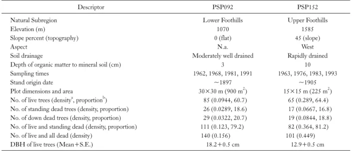
Table 1. Site and stand characteristics of permanent sample plots (PSP) of lodgepole pine
Descriptor PSP092 PSP152
Natural Subregion Lower Foothills Upper Foothills
Elevation (m) 1070 1585
Slope percent (topography) 0 (flat) 45 (slope)
Aspect N.a. West
Soil drainage Moderately well drained Rapidly drained
Depth of organic matter to mineral soil (cm) 3 10
Sampling times 1962, 1968, 1981, 1991 1963, 1976, 1983, 1993
Stand origin date ~1897 ~1905
Plot dimensions and area 30×30 m (900 m2) 15×15 m (225 m2)
No. of live trees (densitya, proportionb) 85 (0.0944, 60.7) 65 (0.289, 64.4) No. of standing dead trees (density, proportion) 26 (0.0289, 18.6) 17 (0.0667, 16.8) No. of down dead trees (density, proportion) 29 (0.0322, 20.7) 19 (0.0844, 18.8) No. of live and standing dead (density, proportion) 111 (0.123, 79.2) 82 (0.364, 81.2)
No. of live and all dead (density) 140 (0.156) 101 (0.449)
DBH of live trees (Mean+S.E.) 18.2+0.5 cm 12.9+0.5 cm
adensity=no. m-2; bproportion (%) is relative to number of live and all dead.
Fig. 1. Spatial point pattern distribution of lodgepole pine in permanent sample plot (PSP) 092 located in the Lower Foothills natural subregion.
The symbol for live trees (open circle) is scaled to diameter at breast height (DBH) of live trees. Dead trees=solid circle.
SW corner of the plot.
Further site and stand characteristics of the two plots are summarized in Table 1. PSP092 in the Lower Foothills is characteristically flat and moderately well drained and or- iginated in the late 1890s. The total number of mapped live (85) and dead standing (26) trees in PSP092 was 111.
PSP152 located in the Upper Foothills has a sloping top- ography with a western facing aspect, is rapidly drained and
originated in the early 1900s. The total number of mapped live (65) and dead standing (17) trees in PSP152 was 82.
Regardless of what category of a tree is considered, PSP152 is noticeably much more dense than PSP092. Furthermore, concomitant with the higher density, the trees in PSP152 also had a lower DBH than trees in PSP092. The spatial point pattern distribution of live and standing dead trees in PSP092 and PSP152 are shown in Figs. 1 and 2, respectively.
Spatial statistical techniques to analyze marked spa- tial point patterns
There are a number of spatial statistical techniques to test the random mortality hypothesis. They can be generally grouped into two categories (Ripley 1981; Kenkel 1988;
Cressie 1993; He and Duncan 2000; Baddeley and Turner 2004; Grey and He 2009; Law et al. 2009): 1) univariate, and 2) bivariate. Univariate analyses were applied to three data sets: (1) live and standing dead, (2) only live, and (3) only standing dead. In addition, bivariate analyses were also conducted to examine the spatial interrelationship between live and standing dead individuals. Most of the analysis of mapped point patterns requires the use of Monte Carlo simulations to examine the significance of any departure of the observed spatial pattern from complete spatial random- ness (CSR) or random mortality. This is described further in the section on constructing random confidence envelopes.
Clark-Evans nearest neighbor statistic (R)
The first univariate analysis includes a modified version of Clark-Evans nearest neighbor statistic taking into ac- count for edge effects (Clark and Evans 1954; Ripley 1981;
Kenkel 1988; Cressie 1993). The nearest neighbor index (R) is defined as: R=
, where rA is the average distance between randomly selected plants and their nearest neigh- bor, and rE is the expected mean distance between nearest neighbors under the null hypothesis of CSR. Values of R>
1 indicate a regular distribution, R=1 indicates a random distribution, and R<1 indicates an aggregated distribution Univariate and bivariate nearest neighbor distribution function (G(r))
The second univariate method examines the cumulative distribution function of nearest neighbors (G(r)) which provides a more detailed analysis of nearest neighbor dis- tances than that provided by the Clark-Evans statistic which can only provide summary information (Ripley 1981; Kenkel 1988; Cressie 1993; Baddeley and Turner 2004; He and Duncan 200). G(r) is the probability that the distance of a randomly chosen plant to its nearest neighbor is equal to or less than r. G(r) has the form of: G(r)observed=
≤ , where ri is the nearest neighbor distance from a randomly chosen plant i, n is the number of events, I(ri <r) is an indicator function such that I(ri<r) = 1 if (ri< r) is true, otherwise I(ri<r)=0. The univariate G(r) func- tion can be extended to the bivariate case to examine the probability that the distance from a typical point of live to nearest dead tree is equal to or less than r, and vice versa.
Univariate (bivariate) G(r)>0 indicates an aggregated dis- tribution (attraction), G(r)=0 indicates a random dis- tribution (independence), and G(r)<0 indicates a regular distribution (repulsion). In either the univariate or bivariate case of G(r), whether the deviation of the observed pattern from CSR or random mortality is significant is assessed us- ing Monte Carlo simulations.
Univariate and bivariate second-order statistic (L(r)) The third univariate technique involves the use of sec- ond-order spatial statistics which unlike the G(r) function examines all plant-to-plant distances and thus provides fur- ther insight into the underlying spatial pattern. A com- monly used function to analyze spatial point patterns is the K-function (K(r)) also known as Ripley’s K-function (Ripley 1981; Kenkel 1988; Cressie 1993; He and Duncan 2000; Baddeley and Turner, 2004; Grey and He 2009; Law et al. 2009). K(r) is also known as a second-moment meas- ure since instead of the mean of the point pattern, the focus of analysis is the variation of the point-point distances. K(r) is defined as as: K(r) = - E (number of other events with- in a distance r of an arbitrary chosen event), where E is the expectation operator. K(r) is usually expressed as L(r):
L(r)=
−r, since the square root transformation helps stabalize the variance. Under the null hypothesis of CSR: E(L(r))=0, such that L(r)>0 suggests an ag- gregated pattern, L(r)=0 suggests a random pattern, and L(r)<0 suggests a regular spatial pattern.
The univariate K-function can be extended to the bi- variate case by taking into account any marks of the point patterns. The bivariate K-function (K12(r)) is defined as:
K12(r) = - E (number of type 2 events within a distance r of an arbitrary event of type 1). K12(r) is usually expressed as L12(r)=
−r. Under the null hypothesis of CSR:
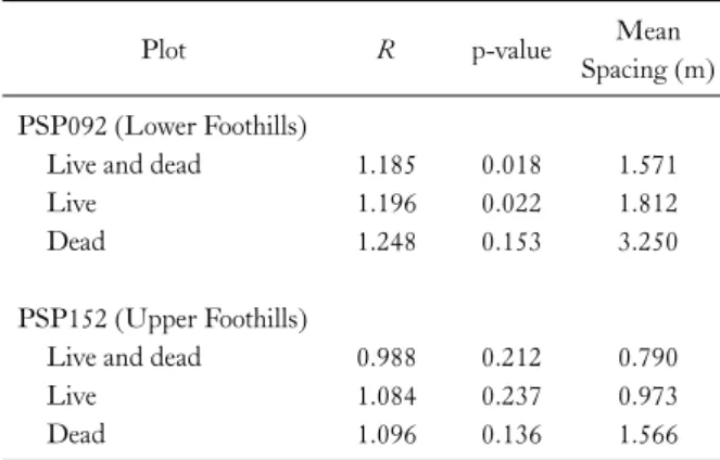
Table 2. Clark-Evans nearest neighbor index (R) statistics for lodgepole pine permanent sample plots
Plot R p-value Mean
Spacing (m) PSP092 (Lower Foothills)
Live and dead 1.185 0.018 1.571
Live 1.196 0.022 1.812
Dead 1.248 0.153 3.250
PSP152 (Upper Foothills)
Live and dead 0.988 0.212 0.790
Live 1.084 0.237 0.973
Dead 1.096 0.136 1.566
E(L12(r))=0, such that L12(r)>0 suggests attraction, L12(r)=0 suggests independence, and L12(r)<0 suggests repulsion. In either the univariate or bivariate case of L(r), whether the deviation of the observed pattern from CSR or random mortality is significant is assessed using Monte Carlo simulations.
Random confidence envelopes
Monte Carlo simulations with 25 iterations were con- ducted to determine whether the spatial patterns deviated from a pattern expected under two null hypotheses of spa- tial randomness (Goreaud and Pelissier 2003). The first null hypothesis (Ho1) is CSR. Using a uniform random number generator, random coordinates were generated for a number of points equivalent to the number of trees in the data set of interest (i.e., both live and dead (univariate, bi- variate cases), only live, and only dead). For each iteration of each random spatial point pattern, the spatial functions (i.e., G(r), K(r), and g(r)) were calculated for each distance r. An approximate 95% confidence envelope was defined as the lowest and highest values of the simulations of the spa- tial functions at each distance r.
The second null hypothesis (Ho2) is random mortality which states that the pattern of surviving trees does not dif- fer from what is expected if mortality is a random event.
Again, using a uniform random number generator, a ran- dom number was applied to each tree in the data set of live and dead trees. The trees were subsequently ranked in as- cending order according to their random numbers, and starting with the minimum ranked random number up to the number of points corresponding to the number of only live or only dead trees were retained. In the bivariate case, the data of live and dead trees was essentially randomly split to the first set of randomly ranked numbers to one category and the second set of randomly ranked numbers to another category. After the random selection of trees, the spatial functions were calculated. An approximate 95% confidence envelope was defined as the lowest and highest values of the simulations of the spatial functions at each distance r.
Implementation of spatial statistical techniques us- ing r functions
The spatial data analysis was conducted in the R stat- istical environment (Venables et al. 2004) using the func-
tions developed by Baddeley and Turner (2004) in their
“spatstat” library extension that includes: clarkevans, Gest (univariate G(r)), Gmulti (bivariate G(r)), Kest (univariate K(r)), and Kmulti (bivariate K(r)). G(r) was estimated us- ing the Kaplan-Meier estimator (Baddeley and Turner 2004). K(r) was estimated using Ripley’s isotropic edge correction (Baddeley and Turner 2004).
Results
Clark-evans nearest neighbor statistic (R)
For PSP092, the Clark-Evans nearest neighbor statistic (R) indicated that the distribution of both alive and dead trees was significantly regular (R=1.185, p=0.018) with a mean spacing between nearest neighbors of 1.571 m (Table 2). The distribution of only live trees was also significantly regular (R=1.196, p=0.022) with a mean spacing of 1.812 m. The distribution of dead trees did not deviate from CSR (R=1.248, p=0.153) with a mean spacing of 3.250 m.
For PSP152, the nearest neighbor index for both live and dead, only live, and only dead, did not deviate sig- nificantly from CSR. Live and dead trees had a mean spac- ing of 0.790 m, while only live trees had a mean spacing of 0.973 m, and only dead trees had a mean spacing of 1.566 m.
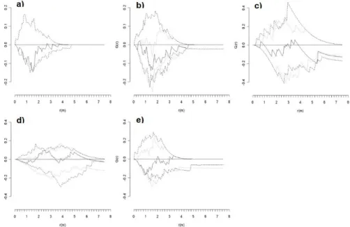
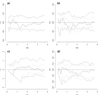
Nearest neighbor distribution function (G(r)) For PSP092, the cumulative distribution function of nearest neighbor distances for live and dead trees was sig- nificantly regular with respect to Ho1 at distances of 1.0,
Fig. 3. Plot 092 in Lower Foothills: Univariate nearest-neighbor distribution function (G(r)=G(r)observed−G(r)theoretical) for three data sets: (a) live and dead trees, (b) live trees, and (c) dead trees. Bivariate G(r) measuring the distance (d) from a typical point of live to nearest dead tree, and (e) from dead to nearest live tree. Univariate (bivariate) G(r) > 0 indicates an aggregated distribution (attraction), G(r) = 0 indicates a random distribution (independence), and G(r) < 0 indicates a regular distribution (repulsion). Observed distribution (__) and confidence envelopes for 25 Monte Carlo simulations for the null hypothesis of complete spatial randomness (- - -) or random mortality (…).
and 1.5-1.6 m (Fig. 3a). Similarly, live trees had a random pattern according to Ho1, but were significantly regular than that expected under Ho2 at 2.9-3.0 m and 3.8-4.5 m (Fig. 3b). Dead trees were also significantly regular com- pared to both Ho1 at 5.4 m, and Ho2 at 5.0-5.4 m and 5.7-7.5 m (Fig. 3c). The bivariate relationship of live to nearest dead tree was that of independence under Ho1, but that of significant attraction under Ho2 at 2.2-2.7 m (Fig.
3d). The relationship of dead to nearest live tree was that of significant repulsion compared to both Ho1 at 1.0 m and Ho2 at 0.9-1.0 m (Fig. 3e).
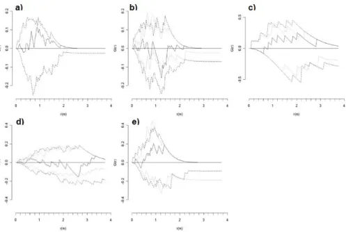
For PSP152, G(r) of live and dead trees did not differ significantly from that expected under Ho1 (Fig. 4a). G(r) of live trees was random under Ho1, but significantly regu- lar compared to Ho2 at 1.1-1.4 m (Fig. 4b). G(r) of dead trees was random under Ho1, but significantly clumped than that expected under Ho2 at 2.0-2.1 m (Fig. 4c). The bivariate relationship between live to nearest dead was that of independence under Ho1, but that of significant re- pulsion under Ho2 at 2.5-2.6 m (Fig. 4d). The bivariate re- lationship of dead to nearest live tree did not deviate from that expected under either Ho1 or Ho2 (Fig. 4e).
Second-order statistic (L(r))
For PSP092, the empirical second-order statistic (L(r)) of live and dead trees showed a significant regular dis- tribution under Ho1 at 0.8 m, but became significantly ag- gregated at distances of 4.9-5.2 m and 5.5-6.2 m (Fig. 5a).
L(r) of live trees showed a significant regular distribution for both Ho1 at 1.6-1.7 m and 2.1-2.7 m, and Ho2 at 2.4-3.2 m (Fig. 5b). L(r) of dead trees was significantly clumped than expected under both Ho1 at distances of 4.3-4.4 m and Ho2 at distances of 4.5-4.7 m (Fig. 5c). The bivariate inter- relationship between live and dead trees showed that there was significant repulsion under Ho1 at 0.8-1.0 m, and sig- nificant attraction than that expected under Ho2 at 2.4-2.5 m (Fig. 5d).
For PSP152, L(r) of live and dead trees was within the confidence evelope defined by Ho1 (Fig. 6a). L(r) of live trees was significantly regular under Ho1 at distances of 1.1-1.4 m, but was within the confidence envelope defined by Ho2 (Fig. 6b). Dead trees were randomly distributed under Ho1, but significantly clumped than expected under Ho2 at 2.0-2.1 m (Fig. 6c). The bivariate L(r) of live and
Fig. 4. Plot 152 in Upper Foothills: Univariate nearest-neighbor distribution function (G(r)=G(r)observed−G(r)theoretical) for three data sets: (a) live and dead trees, (b) live trees, and (c) dead trees. Bivariate G(r) measuring the distance (d) from a typical point of live to nearest dead tree, and (e) from dead to nearest live tree. Univariate (bivariate) G(r)>0 indicates an aggregated distribution (attraction), G(r)=0 indicates a random distribution (independence), and G(r) < 0 indicates a regular distribution (repulsion). Observed distribution (__) and confidence envelopes for 25 Monte Carlo simulations for the null hypothesis of complete spatial randomness (- - -) or random mortality (…).
Fig. 5. Plot 092 in Lower Foothills: Univariate second-order statistic (L(r)) for three data sets: (a) live and dead trees, (b) live trees, and (c) dead trees. (d) Bivariate L(r) measuring the relationship between live and dead trees. Univariate (bivariate) L(r)>0 indicates an aggregated distribution (attraction), L(r)=0 indicates a random distribution (independence), and L(r)<0 indicates a regular distribution (repulsion). Observed distribution (__) and confidence envelopes for 25 Monte Carlo simulations for the null hypothesis of complete spatial randomness (- - -) or random mortality (…).
Fig. 6. Plot 152 in Upper Foothills: Univariate second-order statistic (L(r)) for three data sets: (a) live and dead trees, (b) live trees, and (c) dead trees. (d) Bivariate L(r) measuring the relationship between live and dead trees (d). Univariate (bivariate) L(r)>0 indicates an aggregated distribution (attraction), L(r)=0 indicates a random distribution (independence), and L(r)<0 indicates a regular distribution (repulsion). Observed distribution (__) and confidence envelopes for 25 Monte Carlo simulations for the null hypothesis of complete spatial randomness (- - -) or random mortality (…).
dead trees was within the confidence envelope defined by either Ho1 or Ho2.
Discussion
In the Lower Foothills plot (PSP092) of the current study, there was evidence to suggest regularity in the live plus standing dead trees as indicated by Clark-Evans near- est neighbor index (R), the nearest neighbor distribution function (G(r)) and second-order cumulative distribution function (L(r)) at very local distances. In contrast, instances of clumping were shown by L(r) at larger spatial scale. This regularity in the live plus dead trees was not expected. The results suggest that the stand was initially very regular but the regularity may also be an artifact of not accounting for the down dead trees in the forest inventory.
In the Lower Foothills plot (PSP092), despite the initial local regularity as indicated by G(r) and L(r) of live and dead trees, live trees also showed regularity but at larger spatial scales. Clark-Evans nearest neighbor index also in-
dicated regularity in the spatial pattern of live trees.
Furthermore, in the case of L(r), regularity was more than expected under both Ho1 and Ho2. This indicates that there was some increase in the competitive influence zone of live trees from the initial distribution of live and dead trees. In PSP092, dead trees did not show an expected clumped pat- tern of nearest neighbor distances. Nonetheless, there was clumping observed according to L(r) (for both Ho1 and Ho2) suggesting increased mortality in high density patches.
In terms of the bivariate relationship of live and dead trees in PSP092, there was significant attraction according to G(r) and L(r) under Ho2. This supports the hypothesis that there is mainly one-sided competition for light in this stand. This was expected because of the shade intolerant na- ture of lodgepole pine as well as its tendency to form root grafts (Fraser et al. 2006).
In the Upper Foothills plot (PSP152), the initial dis- tribution of live and dead trees was within random expect- ation according to G(r) and L(r). In contrast, live trees
were significantly regular under Ho2 according to G(r).
According to L(r), live trees were significantly regular un- der Ho1. There is thus some evidence to suggest that there is increased regularity in the surviving members of the stand due to competition. Under Ho2, dead trees were sig- nificantly clumped according to G(r) and L(r) suggesting that dead trees experienced mortality in high density patches. The bivariate relationship between live and dead trees was mainly that of repulsion according to G(r) under Ho2, suggesting two-sided competition for soil nutrients and water in high density patches.
The general pattern of regularity observed in the two plots of lodgepole pine examined in this study has also been observed in other studies that have tested the random mor- tality hypothesis. This spatial pattern of regularity is more likely to occur in species that are shade intolerant. Shade in- tolerant, pioneer tree species undergo self-thinning which often leads to regularly spaced survivors. For instance, Kenkel (1988) examined a stand of shade intolerant jack pine (Pinus banksiana Lamb.) and reported that the initial distribution of live and dead trees was random while the distribution of surviving trees was significantly regular.
The likelihood of regularity to be observed in the spatial pattern of forest stands appears to be also associated with older stands. For instance, both intraspecific and inter- specific competition was observed to influence the spatial point-pattern of shade intolerant Douglas fir (Pseudotsuga menziesii Mirb.) in an old-growth forest stand in British Columbia, Canada (He and Duncan 2000). Density-de- pendent, intraspecific competition was the main driver of stand development at different successional stages in the boreal forest region of Alberta, Canada (Gray and He 2009). Furthermore, Gray and He (2009) observed that the effect of intraspecific competition was initially stronger for early successional species (i.e., trembling aspen (Populus tremuloides) and balsam poplar (Populus balsamifera)) at the early successional stage and intraspecific competition was stronger for late successional species (i.e., white spruce) at the late successional stand stage. In a jack pine stand in Canada, the spatial pattern of live trees was initially clus- tered during the early phases of stand development and then showed very limited regularity at one site later on in stand development (Metsaranta and Lieffers 2008).
Nevertheless, not all studies have examined significant
regularity in the spatial point-pattern of surviving trees. For instance, Kreutz et al. (2015) observed in the boreal forest of Fennoscandia that stands containing Picea abies, Betula pubescens, and Betula pendula, were either randomly dis- tributed or clumped. Kruetz et al. (2015) attributed the clumped pattern to facilitative mechanisms related to nu- trient availability and microclimatic moderation. Furthermore, Little (2002) reported no evidence of density-dependent spatial point-patterns in a boreal mixedwood site containing trembling aspen and jack pine but the lack of density de- pendence may be associated with the young (21-year old) stand that was investigated.
Spatially explicit studies of stands dominated by a single species have shown differences in the spatial pattern of mor- tality that appears to be influenced by species’ shade toler- ance, stand age, and disturbance regime. It is generally ex- pected that shade intolerant, pioneer species experience higher mortality in high density patches. Mortality in lodgepole pine (a shade intolerant species) observed in the current study generally had a tendency towards a clumped spatial pattern. Furthermore, for another shade intolerant species of jack pine examined in western Canada, the spatial pattern of dead trees was initially clustered but over time as the stand aged, the pattern was randomly distributed (Metsaranta and Lieffers 2008). Metsaranta and Lieffers (2008) indicated that after the peak rate of mortality had passed, other factors besides competition were influencing forest dynamics. The likelihood of randomness observed in the spatial pattern of mortality appears to be more likely for tree species sampled in older stands. For instance, Aakala et al. (2012) found that mortality in an old-growth stand of red pine (Pinus resinosa, which is moderately shade toler- ant) in northern Minnesota was spatially random using both Ripley’s K-function and the pair correlation function.
The spatial pattern of mortality events was also predom- inantly random in another old-growth stand (with stand ages up to 209 years) of red pine sampled in Minnesota (Silver et al. 2013). Silver et al. (2013) attributed mortality to multiple agents including windthrow, root-rot fungi, and infrequent droughts. In study and other studies examining shade intolerant tree species establishing after a stand-re- placing fire(e.g., Metsaranta and Lieffers 2008), a clumped spatial pattern in mortality is more likely to occur in a stand replacement fire regime. In contrast, Aakala et al. (2012)
observed random mortality patterns in old growth red pine stands which generally experience a more variable pattern and intensity of repeated surface fires in an understory fire regime.
Conclusions
This study provides new insight and understanding of the underlying competitive processes driving forest stand dynamics of lodgepole pine derived from the analysis of spatial point-patterns. While other spatial ecology studies have devoted attention to other tree species (e.g., jack pine, red pine, trembling aspen), our study represents the first consideration of lodgepole pine. Additional analyses on oth- er boreal tree species would be useful in providing further insight into the ecological process behind competition and mortality in boreal forests.
Acknowledgements
We would like to thank Alberta Agriculture and Forestry for providing access to the spatial data, and F. He for pro- viding comments on a previous version of this manuscript.
This study was supported through a number of scholar- ships to the first author: Natural Sciences and Engineering Research Council of Canada (NSERC) Canada Graduate Scholarship (CGS); Alberta Ingenuity Scholarship; Killam Trust Scholarship; and Prairie Adaptation Research Collaborative (PARC) Graduate Scholarship.
References
Aakala T, Fraver S, Palik BJ, D’Amato AW. 2012. Spatially ran- dom mortality in old-growth red pine forests of northern Minnesota. Can J For Res 42: 899-907.
Alberta Environmental Protection. 1994. Natural regions and sub- regions of Alberta. Alberta Environmental Protection, Edmonton.
Alberta Land and Forest Service. 1994. Permanent sample plot field procedures manual. Alberta Forest Service, Edmonton, AB.
Baddeley A, Turner R. 2004. The spatstat package: spatial point pattern analysis, model-fitting and simulation. http://www.
maths.uawa.edu.au/!adrian/spatstat.html https://rdrr.io/cran/spat-
stat/.Accecced November 2015.
Clark PJ, Evans FC. 1954. Distance to nearest neighbor as a meas- ure of spatial relationships in populations. Ecology 35: 445-453.
Cressie NAC. 1993. Statistics for spatial data. John Wiley and Sons, New York, NY.
Fraser EC, Lieffers VJ, Landhäusser SM. 2006. Carbohydrate transfer through root grafts to support shaded trees. Tree Physiol 26: 1019-1023.
Goreaud F, Pélissier R. 2003. Avoiding misinterpretation of biotic interactions with the intertype K12‐function: population in- dependence vs. random labelling hypotheses. J Veg Sci 14:
681-692.
Gray L, He F. 2009. Spatial point-pattern analysis for detecting density-dependent competition in a boreal chronosequence of Alberta. For Ecol Manag 259: 98-106.
He F, Duncan RP. 2000. Density‐dependent effects on tree survival in an old‐growth Douglas fir forest. J Ecol 88: 676-688.
Huang S. 2000. A Growth and Yield Projection System for seed-origin natural and regenerated lodgepole pine stands with- in an ecologically-based, enhanced forest management framework.
Land and Forest Service, Report T/484, Edmonton, AB.
Kenkel NC. 1988. Pattern of self-thinning in Jack pine: testing the random mortality hypothesis. Ecology 69: 1017-1024.
Kreutz A, Aakala T, Grenfell R, Kuuluvainen T. 2015. Spatial tree community structure in three stands across a forest succession gradient in northern boreal Fennoscandia. Silva Fennica 49:
1279.
Law R, Illian J, Burslem DFRP, Gratzer G, Gunatilleke CVS, Gunatilleke IAUN. 2009. Ecological information from spatial patterns of plants: insights from point process theory. J Ecol 97:
616-628.
Little LR. 2002. Investigating competitive interactions from spatial patterns of trees in multispecies boreal forests: the random mor- tality hypothesis revisited. Can J Bot 80: 93-100.
Lotan JE, Critchfield WB. 1990. Lodgepole pine (Pinus contorta Dougl. ex. Loud..). In: Silvics of North America (Burns RM, Honkala BH, eds). United States Department of Agriculture, Washington.
Metsaranta JM, Lieffers VJ. 2008. A fifty-year reconstruction of annual changes in the spatial distribution of Pinus banksiana stands: does pattern fit competition theory? Plant Ecol 199:
137-152.
Ripley BD. 1981. Spatial Statistics. John Wiley and Sons, Hoboken, NJ.
Silver EJ, Fraver S, D’Amato AW, Aakala T, Palik BJ. 2013.
Long-term mortality rates and spatial patterns in an old-growth forest. Can J For Res 43: 809-816.
Venables WN, Smith DM, R Development Core Team. 2004. An introduction to R. Network Theory Limited, Bristol.