Effective Harmony Search-Based Optimization of Cost-Sensitive Boosting for Improving the Performance of Cross-Project Defect Prediction
Duksan Ryu†⋅Jongmoon Baik††
ABSTRACT
Software Defect Prediction (SDP) is a field of study that identifies defective modules. With insufficient local data, a company can exploit Cross-Project Defect Prediction (CPDP), a way to build a classifier using dataset collected from other companies. Most machine learning algorithms for SDP have used more than one parameter that significantly affects prediction performance depending on different values. The objective of this study is to propose a parameter selection technique to enhance the performance of CPDP. Using a Harmony Search algorithm (HS), our approach tunes parameters of cost-sensitive boosting, a method to tackle class imbalance causing the difficulty of prediction. According to distributional characteristics, parameter ranges and constraint rules between parameters are defined and applied to HS. The proposed approach is compared with three CPDP methods and a Within-Project Defect Prediction (WPDP) method over fifteen target projects. The experimental results indicate that the proposed model outperforms the other CPDP methods in the context of class imbalance. Unlike the previous researches showing high probability of false alarm or low probability of detection, our approach provides acceptable high PD and low PF while providing high overall performance. It also provides similar performance compared with WPDP.
Keywords : Cost-Sensitive Boosting, Cross-Project Defect Prediction, Harmony Search, Search-Based Software Engineering, Transfer Learning
교차 프로젝트 결함 예측 성능 향상을 위한 효과적인 하모니 검색 기반 비용 민감 부스팅 최적화
류 덕 산†⋅백 종 문††
요 약
소프트웨어 결함 예측(SDP)은 결함이 있는 모듈을 식별하기 위한 연구 분야이다. 충분한 로컬 데이터가 없으면 다른 회사에서 수집한 데이 터를 사용하여 분류기를 구축하는 교차 프로젝트 결함 예측(CPDP)을 활용할 수 있다. SDP에 대한 대부분의 기계 학습 알고리즘은 서로 다른 값에 따라 예측 성능에 큰 영향을 미치는 하나 이상의 매개 변수를 사용한다. 본 연구의 목적은 CPDP의 예측 성능 향상을 위해 매개 변수 선 택 기법을 제안하는 것이다. Harmony Search 알고리즘을 사용하여, 예측 어려움을 야기하는 클래스 불균형을 해결하는 방법인 비용에 민감한 부스팅의 매개 변수를 조정한다. 분포 특성에 따라 매개 변수 범위와 매개 변수 간의 제한 조건 규칙이 정의되어 하모니 검색 알고리즘에 적용 된다. 제안된 접근법은 15개의 대상 프로젝트를 대상으로 3개의 CPDP 모델과 내부프로젝트 결함 예측(WPDP) 모델을 비교한다. 실험 결과는 제안된 방법이 클래스 불균형의 맥락에서 다른 CPDP 방법보다 성능이 우수하다는 것을 보여준다. 이전의 연구에서는 탐지 확률이 낮거나 오보 가능성이 높았으나 우리의 기법은 높은 PD와 낮은 PF를 제공하면서 높은 전체 성능을 보였다. 또한 WPDP와 비슷한 성능을 제공하였다.
키워드 : 비용민감 부스팅, 교차프로젝트 결함 예측, 하모니 검색, 검색기반 소프트웨어 공학, 전이 학습 1)
※ This research was supported by Basic Science Research Program through the National Research Foundation of Korea (NRF) funded by the Ministry of Education (NRF-2016R1D1A1A09917660, Artificial Intelligence-based Quantitative Quality Prediction and Evaluation Technique for Software Intensive System).
†정 회 원 : KAIST, School of Computing, Research Professor
††비 회 원 : KAIST, School of Computing, Professor Manuscript Received : October 17, 2017
Accepted : December 9, 2017
* Corresponding Author : Duksan Ryu ([email protected])
1. Introduction
Software defect prediction (SDP) is an attractive field of study identifies defective modules. Software quality assurance resources for software inspection and testing are usually limited and thus they should be allocated with caution. Such valuable resources can be allocated effectively to defective modules identified by SDP. With insufficient
local data, a company can take advantage of Cross-Project Defect Prediction (CPDP), a way to construct a classifier using datasets collected from other companies. SDP has been studied on the basis of various machine learning algorithms. Most machine learning algorithms have used more than one parameter that significantly affect prediction performance depending on different values.
On software defect datasets, the ratio between the defective instance and the non-defective instance is not balanced. This problem called class imbalance causes the difficulty of prediction. One of the main methods to address class imbalance is cost-sensitive learning. Cost-sensitive learning indicates that the costs of incorrectly classified errors are non-uniformly treated while building a classification model. In other words, the importance of class identification is differently reflected into misclassification costs. In this context, it is desired for a classifier to produce high performance of the minority class (defect class) without seriously worsening the performance of the majority class (non-defect class) [1]. In cost-sensitive boosting methods, misclassification costs are easily integrated into the weight update formula. Most cost-sensitive boosting algorithms have only taken into account Within-Project (WP) data without external data. Ryu et al. [2] proposed a cost- sensitive boosting method for CPDP that is called Transfer Cost-Sensitive Boosting (TCSBoost) considering class imbalance in CP settings. It extracted additional cost parameters for instances with different distributional characteristics. For different CPDP settings, parameters should be tuned adaptively. If parameters can be adaptively tuned depending on different CPDP settings, predictive performance may be enhanced. In this study, we investigate if our parameter tuning technique based on Harmony Search [3] can provide high predictive performance in CP settings.
We explore the following research questions:
∙ RQ1: Does Harmony Search technique effectively tune parameters of cost-sensitive boosting for CPDP?
∙ RQ2: Can the proposed method provide the predictive performance comparable to within-project defect prediction?
The objective of this research is to present a search- based optimization method effective for CPDP. We propose a novel approach called TCSBoost using Harmony Search (TCSBoost.HS) that tunes parameters of a cost adjustment function that significantly affect the performance of cost- sensitive boosting in CP settings. We use Jureczko datasets [4] for the experiments obtained from PROMISE repository [5]. The parameters assigning the correct/incorrect classifi- cation costs are related to the distributional characteristics and class imbalance. Using such domain knowledge, the size
of the search space is reduced in the steps of initialization, range settings, and relative value settings between param- eters.
To evaluate prediction performance, TCSBoost.HS approach is compared with TCSBoost and other classification techniques in CP and WP settings. We performed a statistical significance test and the effect size test. The experimental results show that TCSBoost.HS provides better defect prediction ability than CPDP models we compared with. In particular, it shows predictive performance similar to WPDP.
As a result, our proposed approach can effectively help to allocate testing or inspection resources on defect-prone modules in CP settings.
The organization of the remaining sections is as follows.
As a background, Harmony Search is explained in section 2.
In section 3, we describe related work covering SDP and parameter tuning. In section 4, the proposed HS based optimization method is described. Section 5 includes the details of the experimental setup. In section 6, the experimental results are explained. In section 7, the threats to validity are covered. In the last section, the conclusion is summarized.
2. Harmony Search
Harmony Search (HS) is a music-inspired meta-heuristic optimization algorithm. HS mimics the process of instrument players searching the best harmony with their experience and repeated practice while improvising. The algorithm is first suggested by Geem et al. [3]. Since then, it has acquired remarkable results in the field of combinatorial optimization.
The fundamental of HS is like a jazz improvisation.
Players try to make a harmony with each other. They tune the pitch of the instruments based on their experiences or randomly to find a better harmony. By this repeated practice, the players reach to the best harmony that can please the audiences.
Under this principle, HS finds the optimal solution of a given problem through the following steps.
1) Initializes a problem and algorithm parameters 2) Initializes a harmony memory
3) Improvises a new harmony 4) Updates the harmony memory 5) Checks a stopping criterion
Table 1 shows the parameters of HS. Harmony Memory Size (HMS) indicates the maximum size of the experiences of players, representing Harmony Memory (HM). Remaining parameters, Harmony Memory Considering Rate (HMCR), Pitch Adjusting Rate (PAR), and Fret Width (FW) are used
Parameter Description Harmony Memory Size
(HMS)
The number of solution vectors simultaneously handled Harmony Memory
Considering Rate (HMCR)
The rate (0≤HMCR≤1) where HS picks one value randomly from HM
Pitch Adjusting Rate (PAR)
The rate (0≤PAR≤1) where HS tweaks the value which was originally picked from memory Maximum Improvisation
(MI) The number of iterations
Fret Width
(FW) The bandwidth of pitch adjustment Table 1. Parameters of a Harmony Search Algorithm
to generate a new harmony. HMCR is a probability of choosing a harmony from HM, and PAR is a probability to adjust the pitch of chosen harmony. FW represents the changing bandwidth of pitch adjustment. MI (Maximum Improvisation) indicates the maximum number of iterations.
Based on the initialized value of HMS, HS generates the candidate solutions and stores them in HM. The fitness of each candidate is calculated by an objective function. Then, a new harmony is created by 3 ways, according to the parameters, HMCR and PAR.
∙ Random Playing: The new candidate solution is randomly generated by the probability of (1-HMCR).
∙ Memory Consideration: The solution is randomly selected from HM by the probability of HMCR and is preserved as it is by the probability of (1-PAR).
∙ Pitch Adjusting: The solution is randomly selected from HM by the probability of HMCR and is adjusted by the probability of PAR.
After a new candidate solution is generated by one of three ways described above, HM is updated. If the new solution has a better objective function value than the value of the worst candidate solution in HM’s objective function, the new one replaces the old one. HS iterates the solution generating and HM updating process until it reaches the preset exit condition or the maximum iteration value.
3. Related Work
3.1 Software Defect Prediction
Software Defect Prediction (SDP) aims at the optimal allocation of software quality assurance resources via the correct identification of defective modules. Most SDP studies are based on machine learning algorithms [6–11]. Not only Within-Project Defect Prediction (WPDP) using local data to build a classifier but also Cross-Project Defect Prediction
(CPDP) using cross-project data to construct a classifier have attracted many researchers.
Zimmermann et al. [12] presented that only 21 among 622 CPDP cases were successful. They asserted that the identification of the data and process characteristics was crucial for dealing with different distributions between the source project and the target project. They also suggested CPDP issues be investigated by more researchers.
Turhan et al. [13] proposed the relevancy filtering method based on the nearest neighbor for CPDP. They indicated that Within-Project (WP) data were more useful to build a classifier compared to Cross-Project (CP) data.
He et al. [14] employed an example selection to deal with CPDP problems. They used 16 distributional characteristics including mode, median, mean, range, and variance for experiments. They asserted that predictive performance was closely related to such distributional characteristics.
Ma et al. [15] studied an approach called Transfer Naïve Bayes (TNB) for CPDP. As a way of measuring the similarity between projects, the range was used. The similarity weights calculated were used for building their proposed model.
Ryu et al. [16] proposed a boosting method for CPDP considering different distributions and class imbalance together. Asymmetric misclassification costs and similarity weights from the distributional characteristics of a source dataset and a target dataset were derived and different resampling mechanisms depending on them were used. The range was used to compute the similarity weights.
Ryu et al. [17] presented an approach called a Hybrid Instance Selection using Nearest-Neighbor (HISNN) method for CPDP with consideration of class imbalance. It adopted a selective learning technique based on local knowledge. If local knowledge is strong enough, k-nearest neighbor insensitive to class imbalance was used to predict defects.
Otherwise, naïve Bayes using global knowledge was used.
Ryu et al. [2] presented a cost-sensitive boosting method for CPDP that is called Transfer Cost-Sensitive Boosting (TCSBoost) considering class imbalance in CP settings. It applied cost-sensitive learning and transfer learning together to CP data. It extracted additional cost parameters for instances with different distributional characteristics.
Canfora et al. [18] presented a genetic algorithm-based multi-objective classification model called a multi-objective defect predictor (MODEP). Their approach aimed to maximize the number of defect-prone modules (effectiveness) whereas minimizing lines of code to be inspected (inspection cost). It allowed classifiers to provide a compromise between two objectives.
Fig. 1. Overall Process of CPDP using Harmony Search Optimization Ryu and Baik [19] proposed multi-objective naïve Bayes
classification techniques with consideration of the class imbalance problem in CP settings. The multi-objective optimization functions were formulated based on class imbalance. The class probability and the feature weights were parameterized and then they are searched by Harmony Search. They showed that their approaches could be applied to various prediction requirements in CP settings.
According to previous CPDP studies, the identification of distributional properties between a source project and a target project played an important role in the success of CPDP. In addition, recent studies showed that the prediction perfor- mance of CPDP can be enhanced by class imbalance learning.
3.2 Parameter Optimization
Harman et al. [20] reviewed various optimization techniques in software engineering including Simulated Annealing, and Genetic Algorithm. The authors presented limitations of Search-Based Software Engineering (SBSE) and methods to overcome them. They asserted that the search space be reduced using domain knowledge whenever possible.
Merler et al. [21] proposed a method to tune the par- ameters of a cost-sensitive boosting algorithm. A bisection method was used to optimize the performance toward the sensitivity and specificity. The weights for negatives and positives are updated differently at each step. But it didn’t address different dataset distributions.
Wang and Yao [22] proposed a variant of AdaBoost.NC [23] using a Negative Correlation learning algorithm. During the training of a boosting algorithm, a parameter was automatically configured. The dynamic version showed
better performance than the original AdaBoost.NC.
Manjarres et al. [24] reviewed application portfolio of the music-inspired Harmony Search algorithm used in various domains including computer science, electrical engineering and civil engineering. They pointed out, as a meta-heuristic algorithm, it was successfully applied to solve computa- tionally expensive optimization problems.
In this study, Harmony Search was applied to optimize the parameters of cost-sensitive boosting for CPDP.
Additionally, it is adjusted to decrement the search space using characteristics of dataset distributions and class imbalance.
4. Harmony Search Based Parameter Optimization
We propose a parameter optimization technique using Harmony Search for Transfer Cost-Sensitive Boosting (TCSBoost) approach. This approach aims to identify optimal parameters and efficiently decreasing the search space by employing domain knowledge drawn from distributional properties and class imbalance. Fig. 1 illustrates the overall defect prediction process using a Harmony Search algorithm.
After the preparation of defect data for training and testing, training data are resampled with SMOTE [25] and Tomek Links [26] to deal with class imbalance. Then, the similarity weight using the range method [16] is calculated and the parameters are tuned via Harmony Search. Next, the TCSBoost model is built and tested using target data.
Finally, the performance of prediction is evaluated with four performance measures.
4.1 Preparing Defect Dataset
Source and target project data are arranged as a training set and a test set respectively. If an example has at least a bug, it is labelled as buggy. If it has no bug, it is labelled as clean.
4.2 Resampling with SMOTE and Tomek Link
SMOTE (Synthetic Minority Over-sampling Technique) [25] and Tomek links [26] are used in our approach to represent the defective instances better. SMOTE, a way of over-sampling the minority class, generates synthetic minority class instances instead of duplicating existing instances. Tomek links can be used to under-sample instances. They only identify instances close to the class boundary. When the majority class instances close to the class boundary are under-sampled, overlapping around the class boundary can be reduced. We performed SMOTE and then Tomek link-based under-sampling. This can increase the performance of the Probability of Detection (PD) although the Probability of a False alarm (PF) increases. PD and PF are explained in detail in the later phase.
4.3 Similarity Weight Computation
In this phase, the similarity weight is computed to identify the distributional characteristics between source data and target data. This method is used in several CPDP studies [2], [15], [16], [27].
Suppose is the jth attribute of , given a sequence
⋯. The maximum and minimum value of jth attribute in the test data are obtained as follows:
max 1, 2, … , , min 1, 2, … , ,
where m is the number of the test instances, k is the number of attributes, and …. The vector
⋯ has the maximum value of the attribute on the test data and the vector ⋯ has the minimum value of the attribute on the test data. Then, the similarity weight of each training instance is calculated by the following:
∑ , (1)
where is the th attribute of instance and
≤ ≤ 4.4 Transfer Cost-Sensitive Boosting TechniqueThe overall process of TCSBoost only excludes the step
of Harmony Search Optimization in Fig. 1. TCSBoost addresses class imbalance between the defect class and the non-defect class as well as feature distributional differences between a source project and a target project. Algorithm 1 shows the TCSBoost algorithm.
Source project data (S), a small amount of target project data (T), and the similarity weight (SW) are input parameters. Firstly, source data and target data are assembled together as a training set. Secondly, the iteration of the boosting algorithm is performed. The data weight vector (wn) is used by the base classifier (h) identifying weighted instances during training.
AdaCost [28] only deals with the class imbalance. By adapting a cost adjustment function for CPDP, TCSBoost addresses not only the class imbalance but also the distributional characteristics. Classification costs are assigned differently according to the similarity between a training set and a test set.
The cost adjustment function, (n) is depicted as (n) =
(sign(tn, hm), cn), where sign(tn, hm) is positive for correct classification (+) and negative for incorrect classification (-).
Distribution Cost adjustment
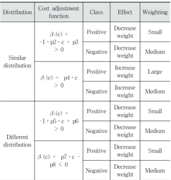
function Class Effect Weighting
Similar distribution
+(c) = -1․p2․c + p3
> 0
Positive Decrease
weight Small Negative Decrease
weight Medium
-(c) = p4․c
> 0
Positive Increase
weight Large Negative Increase
weight Medium
Different distribution
+(c) = -1․p5․c + p6
> 0
Positive Decrease
weight Small Negative Decrease
weight Medium
-(c) = p7․c - p8 < 0
Positive Decrease
weight Small Negative Decrease
weight Medium Table 2. Effect of Cost Adjustment Function The cost adjustment function of TCSBoost is as follows:
∙ The cost adjustment function for the instances with the same or similar distribution
+(c) = -0.25․c + 0.25
-(c) = 0.25․c
∙ The cost adjustment function for the instances with the different distribution
+(c) = -0.25․c + 0.25
-(c) = 0.25․c - 0.5
The previous study proposing TCSBoost demonstrated how small amount of WP data (target project data) can be used together with CP data (source project data) in the boosting algorithm. In order for WP data to be used as training data, more time and efforts for testing and inspection are required to label them as buggy or clean. In this study, however, we build a boosting model using only CP data without including WP data. Thus, our approach can be utilized early without additional efforts.
4.5 Harmony Search-Based Optimization Technique Because the cost adjustment function of TCSBoost mainly affects the defect prediction performance, we aim to optimize its parameters. The parameters to optimize are identified considering class imbalance and distributional characteristics.
Because the cost factor of the minority class is set to 1.0 as Sun et al. did [29], it is not considered as a parameter to tune. The parameter variables identified to tune are from p1 to p8 as follows:
∙ The cost factor of the majority class: p1
∙ The cost adjustment function for the instances with the similar distribution
+(c) = -1․p2․c + p3
-(c) = p4․c
∙ The cost adjustment function for the instances with the different distribution
+(c) = -1․p5․c + p6
-(c) = p7․c - p8
Table 2 shows the effect of a cost adjustment function we adopted in our approach based on the weight update rule of TCSBoost. For the source data belonging to the similar distribution, the weight of instances predicted correctly is decreased and the weight of instances predicted incorrectly is increased. In the case of true prediction, we decrease the weight of True Positives more conservatively than those of True Negatives. In the case of false prediction, the weights of False Negatives are increased more than those of False Positives. For the source data belonging to the different
distribution, we decrease the weight of instances classified correctly and decrease the weight of instances classified incorrectly. In the case of true prediction, the weights of True Positives are decreased more than those of True Negatives. In the case of false prediction, the weights of False Negatives are decreased more conservatively than those of False Positives.
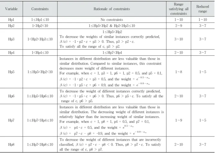
Harman et al. [20] presented SBSE limitations and techniques to overcome them. They guided domain knowledge should be employed whenever possible. In particular, when the fitness function is too computationally expensive, the size of the search space can be efficiently reduced by utilizing domain knowledge. In this study, several parts that domain knowledge can be used are identified. The lower/upper bounds of the variable can be enforced with several constraints drawn from distributional characteristics. Such constraints can help to reduce the size of the search space of a HS algorithm. Rationale of constraints is based on the mechanisms addressing the different correct/incorrect classification costs between the majority class and the minority class, and different distributions between a source project and a target project.
Table 3 defines the search space where HS aims to find an optimal parameter configuration. The above parameters of TCSBoost.HS (i.e., from p1 to p8) have the range in [0,1].
To simplify a HS algorithm, they are replaced into integer values by multiplying 10 (i.e., from Hp1 to Hp8). All variables can have a value ranging from 1 to 10. Based on distributional characteristics, ranges satisfying all constraints
from Hp1 to Hp8 can be obtained. We further reduce the range considering the constraints and the properties of the parameters. Compared to the other parameters, Hp5 and Hp7 need to have smaller values, so the range from 1 to 5 is chosen. The other values are selected with the middle range (from 3 to 7) because high value of each parameter can increase/decrease the weight significantly during iteration and may cause overfitting.
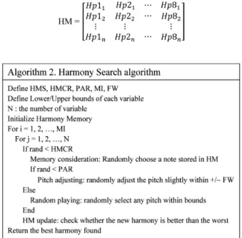
Algorithm 2 describes the Harmony Search algorithm.
After the parameters of HS are defined, Harmony Memory (HM) is initialized before running the main loop.
It has the following form in the case of the seven variables and HMS = n.
Originally, the entries of HM are randomly configured. In our experiments, as part of decreasing the search space, HM is initialized like the following:
The initialization of HM is crucial to reduce the size of the search space because initial parameter values act as a baseline of the performance. By considering different impacts of class imbalance of each dataset, the whole range of Hp1 is covered. The chosen values of the remaining
parameters (from Hp2 to Hp8) are based on constraints derived from the distributional properties between a training set and a test set. They are the median values of the reduced range in Table 3.
Memory consideration means that the algorithm randomly selects a note stored in HM with the probability of 1-PAR. Pitch adjusting indicates that the algorithm randomly adjusts the pitch slightly within +/- FW. It should ensure that constraints and lower/upper bounds are satisfied. Random playing indicates that the algorithm randomly selects any pitch within lower/upper bounds.
Constraints and lower/upper bounds are checked to be satisfied. In the Harmony Memory update step, the algorithm checks whether the new harmony drawn from the above methods is better than the worst. Finally, the algorithm returns the best harmony stored in HM.
As a fitness function, we compute the weighted geometric mean (WG-mean) value after running TCSBoost with the eight parameters. WG-mean is explained in the phase of performance report in detail. At this time, source project data are divided into training data and validation data.
To select validation data, we employed the technique used by Ryu et al. [16]. In this method, source instances similar to target data are intended to be evenly distributed into the training set and the validation set. The process of the validation data selection is shown in Fig. 2. (1) Input data are split in 50:50 randomly. (2) Each half set is sorted by the weight in descending order and data with the high weight are chosen as validation data. Two fifth of a half set are chosen for validation data. Thus, a fifth of the total input data are employed as a validation set. The remaining instances are chosen as a training set.
The entire source project data and the parameters identified after the optimization are used as input data for building a final TCSBoost model.
Fig. 2. Validation Data Selection
4.6 Classification Prediction
In this phase, using the previously built boosting model, each instance of target project data is classified as buggy or clean. The feature space of target data is identical to that of source data.
Variable Constraints Rationale of constraints
Range satisfying all
constraints
Reduced range
Hp1 1≤Hp1≤10 No constraints 1~10 1~10
Hp2 1<Hp2<10 1≤Hp5<Hp2 & Hp2<Hp3≤10 2~9 3~7
Hp3 1<Hp2<Hp3≤10
1≤Hp5<Hp2
To decrease the weights of similar instances correctly predicted,
+(c) = -1․p2․c + p3 > 0. Thus, p3 > p2․c.
To satisfy all the range of c, p3 > p2.
3~10 3~7
Hp4 1<Hp4≤10 1≤Hp7<Hp4 2~10 3~7
Hp5 1≤Hp5<Hp2<10
Instances in different distribution are less valuable than those in similar distribution. Compared to similar instances, this constraint decreases more weight of different instances.
For example, when c = 1, p3 = 1, p6 = 1, p2 = 0.5, and p5 = 0.1,
+(c) = -1․p2․c + p3 = 0.5, and the weight = ⋅
+(c) = -1․p5․c + p6 = 0.9, and the weight = ⋅
1~8 1~5
Hp6 1≤Hp5<Hp6≤10
To decrease the weight of different instances correctly predicted,
+(c) = -1․p5․c + p6 > 0. Thus, p6 > p5․c. To satisfy all the range of c, p6 > p5.
2~10 3~7
Hp7 1≤Hp7<Hp4≤10
Instances in different distribution are less valuable than those in similar distribution. The decreasing weight of different instances is relatively higher than the increasing weight of similar instances.
For example, when c = 1, p8 = 1, p4 = 0.5, and p7 = 0.1,
-(c) = p4․c = 0.5, and the weight = ⋅
-(c) = p7․c - p8 = -0.9, and the weight = ⋅
1~9 1~5
Hp8 1≤Hp7<Hp8≤10
To decrease the weight of different instances that are incorrectly classified, -(c) = p7․c - p8 < 0. Thus, p8 > p7․c. To satisfy all the range of c, p8 > p7.
2~10 3~7
Table 3. Parameter for Optimization
Predicted class
Buggy Clean
Actual class
Buggy TP (True Positive) FN (False Negative) Clean FP (False Positive) TN (True Negative)
Table 4. Confusion Matrix 4.7 Performance Report
Software defect datasets tend to have the class imbalance issue. The learner constructed on such datasets is mostly evaluated by the overall and individual performance together.
The individual performance on the defect class is typically assessed by the Probability of Detection (PD) and the Probability of a False alarm (PF). Table 4 shows a confusion matrix. True Positive (TP) is the number of buggy instances predicted correctly as buggy. False Positive (FP) is the number of clean instances predicted as buggy. True Negative (TN) is the number of clean instances predicted correctly as clean. False Negative (FN) is the number of buggy instances predicted as clean. PD indicates the ratio of appropriate instances among all the retrieved instances.
PD is defined as:
. PF represents the
proportion of clean instances predicted as buggy. PF is defined as:
. The lower PF value is better in contrast to PD.
Geometric mean (G-mean) and Balance are useful for assessing the overall performance of predictors under the imbalanced context. Balance is a Euclidean distance from the ideal point (PD=1, PF=0) to real (PD, PF) point. Balance is defined as:
. G-mean indicates the geometric mean of recall values from the non-defect class and the defect class. G-mean is described as: G-mean = . They aim to show how well a classifier can balance the performance between the clean class and the buggy class. In contrast to PF, three metrics including PD, Balance and G-mean are better when they are higher.
WG-mean = where WPD and W1-PF are the weight for PD and 1-PF respectively. For instance, suppose WPD = 2 and W1-PF = 1, WG-mean = . PD has greater value than
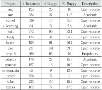
Project # Instances # Buggy % Buggy Description
ant 125 20 16 Open-source
arc 234 27 11.5 Academic
camel 339 13 3.8 Open-source
e-learning 64 5 7.8 Academic
jedit 272 90 33.1 Open-source
log4j 135 34 25.2 Open-source
lucene 195 91 46.7 Open-source
poi 237 141 59.5 Open-source
prop-6 660 66 10 Proprietary
redaktor 176 27 15.3 Academic
synapse 157 16 10.2 Open-source
systemdata 65 9 13.8 Open-source
tomcat 858 77 9 Open-source
xalan 723 110 15.2 Open-source
xerces 162 77 47.5 Open-source
Table 5. Projects in the Jureczko Dataset
Features
weighted methods per class (WMC), depth of inheritance tree (DIT), number of children (NOC), coupling between object classes (CBO), response for a class (RFC), lack of cohesion in methods (LCOM), lack of cohesion in methods (LCOM3), number of public methods (NPM), data access metric (DAM), measure of aggregation (MOA), measure of functional abstraction (MFA), cohesion among methods of class (CAM), inheritance coupling (IC), coupling between methods (CBM), average method complexity (AMC), afferent couplings (Ca), efferent couplings (Ce), maximum McCabe’s cyclomatic complexity (Max(CC)), average McCabe’s cyclomatic complexity (Avg(CC)), lines of code (LOC)
Table 6. Features of the Jureczko Datasets 1-PF in the context of class imbalance. In line with this,
WG-mean allows us to give more weights to PD while tuning the parameters of TCSBoost.
5. Experimental Setup
We answer the two research questions by conducting the comparative experiments. In order to figure out the effec- tiveness of using WG-mean, the experiments are performed with different weights of PD and 1-PF, i.e. 1.0:1.0 and 1.2:1.0 respectively. Our approaches are compared with Na?ve Bayes, Naive Bayes with a k-Nearest Neighbor filter [13]
and TCSBoost under CP settings for RQ1. For RQ2, we investigate if the performance of our method is similar to that of Naive Bayes under WP settings.
Jureczko datasets are used to compare our method with other classifiers, because they are popularly used in the SDP studies. Balance and G-mean are effective performance metrics under the imbalanced context, because they are computed with the values of both PD and PF. The overall performance (e.g., Balance and G-mean) and the defect detection rate (PD) have a trade-off relationship [22].
Therefore, it is crucial to obtain a classifier producing high accuracy for the minority class while the accuracy of the majority class is not severely lowered. We formulate the following hypotheses to answer RQ1 and RQ2.
∙ H10: The performance of TCSBoost.HS is not better than those of other CPDP methods.
∙ H1A: The performance of TCSBoost.HS is better than those of other CPDP methods.
∙ H20: The performance of TCSBoost.HS is not similar to that of within-project defect prediction.
∙ H2A: The performance of TCSBoost.HS is similar to that of within-project defect prediction.
5.1 Datasets for Experiments
The Jureczko datasets [4] contain the instances represented with 20 static code attributes and 1 class label indicating whether the instance is defective or non-defective. 15 datasets were chosen from PROMISE repository [5] as Ryu et al. [2]
did. They contain 11 open-source projects, 3 academic projects and a proprietary project. In Table 5, the properties of each project are explained. Table 6 shows the list of features of the Jureczko datasets used in the experiments.
5.2 CPDP and WPDP Settings
A dataset was chosen to be target data (for testing). The remaining datasets were utilized as source data (for training).
Each experiment of CPDP was conducted 30 times, iteratively.
For WPDP settings, a stratified M x N (M=6, N=5) fold cross validation strategy is employed.
5.3 Classification Models
In the cases of TCSBoost and TCSBoost.HS, Naive Bayes is used as a base learner. We used the implementation of the WEKA machine learning toolkit [30]. All of training and test data were min-max normalized, indicating that the range of features is rescaled to scale the range in [0, 1].
To compare the predictive performance, we included other learning algorithms, i.e., Naive Bayes under CP settings (CP NB), Naive Bayes with a kNN filter (CP NB+NN) and Naive Bayes under WP settings (WP NB). Naive Bayes is selected because it generally produces high prediction performance in Software Defect Prediction studies [6]. A log-filter was applied to training and test data before running the three models.
5.4 Parameter Setup
In the boosting algorithm, an empirical user-defined parameter, Lambda (λ), is utilized for the penalty magnitude
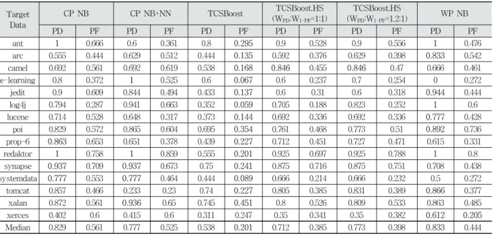
Target Data
CP NB CP NB+NN TCSBoost TCSBoost.HS
(WPD:W1-PF=1:1)
TCSBoost.HS
(WPD:W1-PF=1.2:1) WP NB
PD PF PD PF PD PF PD PF PD PF PD PF
ant 1 0.666 0.6 0.361 0.8 0.295 0.9 0.528 0.9 0.556 1 0.476
arc 0.555 0.444 0.629 0.512 0.444 0.135 0.592 0.376 0.629 0.398 0.833 0.542
camel 0.692 0.561 0.692 0.619 0.538 0.168 0.846 0.455 0.846 0.47 0.666 0.461
e-learning 0.8 0.372 1 0.525 0.6 0.067 0.6 0.237 0.7 0.254 0 0.272
jedit 0.9 0.609 0.844 0.494 0.433 0.137 0.6 0.31 0.6 0.318 0.944 0.444
log4j 0.794 0.287 0.941 0.663 0.352 0.059 0.705 0.188 0.823 0.252 1 0.6
lucene 0.714 0.528 0.648 0.317 0.373 0.144 0.692 0.336 0.692 0.336 0.777 0.428
poi 0.829 0.572 0.865 0.604 0.695 0.354 0.761 0.468 0.773 0.51 0.892 0.736
prop-6 0.863 0.653 0.651 0.378 0.439 0.227 0.712 0.451 0.727 0.471 0.615 0.331
redaktor 1 0.758 1 0.859 0.555 0.201 0.925 0.697 0.925 0.788 1 0.8
synapse 0.937 0.709 0.937 0.673 0.75 0.241 0.875 0.716 0.875 0.751 0.708 0.438
systemdata 0.777 0.553 0.777 0.464 0.444 0.089 0.666 0.214 0.666 0.232 0.5 0.272
tomcat 0.857 0.466 0.233 0.23 0.74 0.227 0.805 0.385 0.831 0.389 0.866 0.377
xalan 0.872 0.561 0.936 0.65 0.745 0.451 0.8 0.526 0.809 0.533 0.863 0.485
xerces 0.402 0.6 0.415 0.6 0.311 0.247 0.35 0.341 0.35 0.382 0.612 0.205
Median 0.829 0.561 0.777 0.525 0.538 0.201 0.712 0.385 0.773 0.398 0.833 0.444
Table 8. The Median PD & PF Performance of Classification Models
Parameter Setting
Harmony Memory Size (HMS) 10
Harmony Memory Considering Rate
(HMCR) 0.8
Pitch Adjusting Rate (PAR) 0.4
Maximum Improvisation (MI) 10
Fret Width (FW) 10% of total value
range Table 7. Parameter Setting of Harmony Search
during each repitition. The value of λ is set to 0.5 to simplify the usage of all boosting algorithms. The maximum number of iterations (M) of TCSBoost and TCSBoost.HS algorithms is set to 30. In the TCSBoost algorithm, the cost factor of the minority class is fixed as 1.0. For the majority class, it is set to 0.5. Table 7 describes the parameter values of Harmony Search used for the experiments. Recommended parameter settings [31, 32] are as follows. HMS = 30~100, HMCR = 0.7~0.95, PAR = 0.1~0.5, and FW = 1~10%. In our approach, the value of HMS is set to 10 considering efficiency.
6. Experimental Results
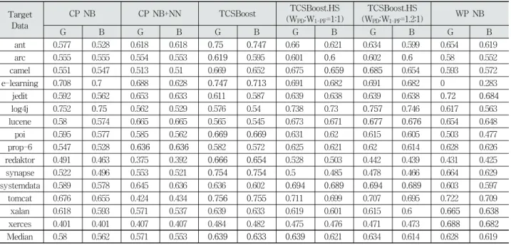
Tables 8 and 9 show PD, PF, G-mean and Balance values of classifiers in CP and WP settings. The best performing cases are marked in boldface.
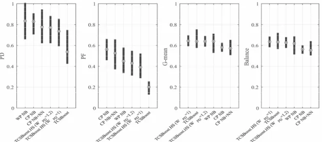
Table 8 describes the median PD and PF values of classifiers. In Fig. 3, a scatter plot is illustrated using median PF and PD values of six classifiers over fifteen datasets. The ideal value of PD and PF is 1 and 0 respectively. As such,
the better classifier has many points located at the bottom right of the regions. While CP NB produces high PD (0.829), it produces the worst PF (0.561). Therefore, Fig. 3 shows most of the points are placed at the top right of the regions.
CP NB+NN filters irrelevant source instances out through the nearest-neighbor filter. This results in reducing PF, but it is still high (0.525). TCSBoost, two TCSBoost.HS models and WP NB show more balanced performance withregards to PD and PF. TCSBoost shows the best PF (0.201) and the worst PD (0.538). Two Harmony Search based approaches show higher PD than TCSBoost while showing worse PF rates. Particularly, when WPD is larger than 1, PD is considerably improved compared to TCSBoost. Two TCSBoost.HS models show worse PD and better PF than WP NB. The practically useful predictor
Fig. 3. Scatter Plot of Median PF & PD Values of Six Classifiers Over 15 Datasets
![Fig. 1. Overall Process of CPDP using Harmony Search OptimizationRyu and Baik [19] proposed multi-objective naïve Bayes](https://thumb-ap.123doks.com/thumbv2/123dokinfo/5255522.630037/4.918.112.807.832.1134/overall-process-harmony-search-optimizationryu-proposed-objective-naïve.webp)