Development of a Combined GPS/GLONASS PPP Method

JPNT 3(1), 31-36 (2014)

http://dx.doi.org/10.11003/JPNT.2014.3.1.031

Copyright © The Korean GNSS Society http://www.gnss.or.kr plSSN: 2288-8187

J ^PNT

Journal of Positioning, Navigation, and Timing

1. INTRODUCTION

A traditional method for providing precise position information is to use the Real Time Kinematic (RTK). In this method, common error terms are eliminated by differencing the data observed at two Global Navigation Satellite System (GNSS) reference stations. To obtain an accurate user position (1 cm level) using the RTK technique, accurate information from at least one reference station is required.

Therefore, for the efficient use of the RTK technique, there should be a GNSS reference station that serves as a reference. Also, if baseline distance increases, positioning accuracy decreases because the common errors that change in space cannot be completely eliminated. In contrast, unlike RTK that is based on differencing, the Precise Point Positioning (PPP) technique is a method which accurately models various error factors that affect navigation signals and which applies error information. PPP can determine precise absolute coordinates. However, in the case of real-

Development of a Combined GPS/GLONASS PPP Method

Byung-Kyu Choi

^1†

, Kyoung-Min Roh

¹

, Sang Jeong Lee

²

1

Astronomy and Space Technology R&D Division, Korea Astronomy and Space Science Institute, Daejeon 305-348, Korea

2

Department of Electronics Engineering, Chungnam National University, Daejeon 305-764, Korea

ABSTRACT

Precise Point Positioning (PPP) is a stand-alone precise positioning approach. As the quality of satellite orbit and clock products from analysis centers has been improved, PPP can provide more precise positioning accuracy and reliability. A combined use of Global Positioning System (GPS) and Global Orbiting Navigation Satellite System (GLONASS) in PPP is now available. In this paper, we explained about an approach for combined GPS and GLONASS PPP measurement processing, and validated the performance through the comparison with GPS-only PPP results. We also used the measurement obtained from the GRAS reference station for the performance validation. As a result, we found that the combined GPS/GLONASS PPP can yield a more precise positioning than the GPS-only PPP.

Keywords: GPS, GLONASS, PPP, performance

time data processing, positioning accuracy is low because precise satellite orbit and clock product needs to be directly calculated or relevant information needs to be received from international GNSS analysis centers (ACs).

The PPP technique using Global Positioning System (GPS) has drawn much attention from many researchers over the past 10 years. As the GLObal NAvigation Satellite System (GLONASS), which is the Russian navigation satellite system, has been recently modernized and 24 GLONASS satellites have been in normal operation in the orbits since late 2011, many studies have been performed on using GLONASS for geodetic survey or navigation. Also, as the orbit and time information of GPS and GLONASS satellites, which is provided from international GNSS ACs, has become more precise, PPP has been widely used in positioning and scientific research. The performance of GPS PPP for positioning has already been explained in a number of papers (Zumberge et al. 1997, Kouba & Héroux 2001, Gao

& Shen 2002, Geng et al. 2010).

Recently, PPP techniques that combined GPS and GLONASS have been introduced in several papers (Tolman et al. 2010, Li et al. 2009). They all explained the use of the combined data processing of GPS and GLONASS satellites, and especially emphasized the use of GLONASS satellite observation data at locations where the visibility of GPS satellites is low (i.e., number of satellites is less Received Jan 20, 2014 Revised Feb 03, 2014 Accepted Feb 04, 2014

†

Corresponding Author E-mail: [email protected]

Tel: +82-42-865-3237 Fax: +82-42-861-5610

http://dx.doi.org/10.11003/JPNT.2014.3.1.031

GNSS Service (IGS) reference stations, Cai & Gao (2007) presented that the positioning accuracy of combined GPS/

GLONASS PPP improved by more than 30% on average compared to that of GPS-only PPP, and that in the case of static positioning, the convergence time was reduced by more than 20%.

In this study, a combined GPS/GLONASS PPP approach was developed, and its performance was compared with that of GPS-only PPP. In addition, the fields, to which a combined GPS/GLONASS PPP can contribute, were discussed.

2. MEASUREMENT PROCESSING APPROACH

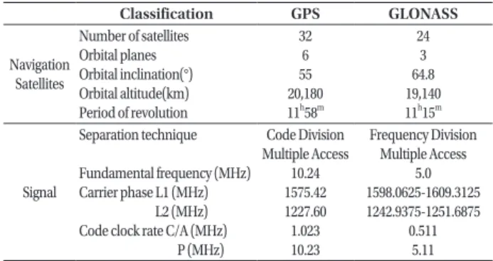
For GLONASS satellites, each satellite uses different frequency, unlike GPS satellites. GPS satellites have unique identification code, while GLONASS identifies satellites using Frequency Division Multiple Access (FDMA), which is a frequency division system. Table 1 summarizes the detailed characteristics of the GPS and GLONASS systems.

GLONASS satellites transmit signals by separating two frequency bands as shown in Eqs. (1) and (2).

( )

1

1602 0.5625 MHz

f

L

= + ´ a (1)

( )

2

1246 0.4375 MHz

f

L

= + ´ a (2)

where a represents the frequency channel number. The frequency channel number can be checked in a GLONASS navigation file.

To obtain precise position information through PPP data processing, dual-frequency (L1 and L2) measurements are required. In other words, this is to eliminate ionospheric error, which is the largest error source in the process of navigation signal transmission, through the linear combination of dual frequencies.

Eq. (3) shows the ionosphere-free linear combinations of carrier (LC) and observed code value (PC), respectively (Hofmann-Wellenhof et al. 2001).

þ ý ü î í

ì

- º

- º

2 2 1 1

2 2 1 1

P C P C PC

L C L C

LC (3)

where L and

₁

L represent the carrier phases with different frequencies; and

₂

P and

₁

P

₂

represent the code phases. The constants, C

1

and C

2

are as follows.

22 12

12

1

f f

C f

= - ,

₂

2 2 1

22

2

f f

C f

= -

The ionosphere-free linear combination of observation information calculated using Eq. (3) can be also expressed as shown in Eq. (4) (Kouba 2003).

e

r + - + + + D +

= c dt dT T N

LC ( ) (4)

where r represents the geometric distance between receiver and satellite; dt and dT represent the time errors of receiver and satellite, respectively; c represents the speed of light; T represents the tropospheric delay; N represents the ionosphere-free linear

(1) (2) where

( )

1

1602 0.5625 MHz

f

L

= + ´ a (1)

( )

2

1246 0.4375 MHz

f

L

= + ´ a (2)

where a represents the frequency channel number. The frequency channel number can be checked in a GLONASS navigation file.

To obtain precise position information through PPP data processing, dual-frequency (L1 and L2) measurements are required. In other words, this is to eliminate ionospheric error, which is the largest error source in the process of navigation signal transmission, through the linear combination of dual frequencies.

Eq. (3) shows the ionosphere-free linear combinations of carrier (LC) and observed code value (PC), respectively (Hofmann-Wellenhof et al. 2001).

þ ý ü î í

ì

- º

- º

2 2 1 1

2 2 1 1

P C P C PC

L C L C

LC (3)

where L and

₁

L represent the carrier phases with different frequencies; and

₂

P and

₁

P

₂

represent the code phases. The constants, C

1

and C

2

are as follows.

22 12

12

1

f f

C f

= - ,

₂

2 2 1

22

2

f f

C f

= -

The ionosphere-free linear combination of observation information calculated using Eq. (3) can be also expressed as shown in Eq. (4) (Kouba 2003).

e

r + - + + + D +

= c dt dT T N

LC ( ) (4)

where r represents the geometric distance between receiver and satellite; dt and dT represent the time errors of receiver and satellite, respectively; c represents the speed of light; T represents the tropospheric delay; N represents the ionosphere-free linear combination of ambiguities; and e represents the measurement error including multipath

represents the frequency channel number. The frequency channel number can be checked in a GLONASS navigation file.

To obtain precise position information through PPP data processing, dual-frequency (L1 and L2) measurements are required. In other words, this is to eliminate ionospheric

of carrier (LC) and observed code value (PC), respectively (Hofmann-Wellenhof et al. 2001).

value (PC), respectively (Hofmann-Wellenhof et al. 2001).

þ ý ü î í

ì

- º

- º

2 2 1 1

2 2 1 1

P C P C PC

L C L C

LC (3)

where L and

1

L represent the carrier phases with different frequencies; and

₂

P and

₁

P

₂

represent the code phases. The constants, C

1

and C

2

are as follows.

2 2 2 1

2

1

f

1

f

C f

= - ,

₂

2 2 1

2

2

f

2

f

C f

= -

The ionosphere-free linear combination of observation information calculated using Eq. (3) can be also expressed as shown in Eq. (4) (Kouba 2003).

e

r + - + + + D +

= c dt dT T N

LC ( ) (4)

where r represents the geometric distance between receiver and satellite; dt and dT represent the time errors of receiver and satellite, respectively; c represents the speed of light; T represents the tropospheric delay; N represents the ionosphere-free linear combination of ambiguities; and e represents the measurement error including multipath error. ^D includes the antenna phase center and variation of satellite and receiver, Earth tide,

(3)

where L

₁

and L

₂

represent the carrier phases with different frequencies; and P

₁

and P

₂

represent the code phases. The constants, C

₁

and C

₂

are as follows.

þ ý ü î í

ì

- º

- º

2 2 1 1

2 2 1 1

P C P C PC

L C L C

LC (3)

where L and

₁

L represent the carrier phases with different frequencies; and

₂

P and

₁

P

₂

represent the code phases. The constants, C

₁

and C

₂

are as follows.

2 2 2 1

12

1

f f

C f

= - ,

₂

2 2 1

22

2

f f

C f

= -

The ionosphere-free linear combination of observation information calculated using Eq. (3) can be also expressed as shown in Eq. (4) (Kouba 2003).

e

r + - + + + D +

= c dt dT T N

LC ( ) (4)

where r represents the geometric distance between receiver and satellite; dt and dT represent the time errors of receiver and satellite, respectively; c represents the speed of light; T represents the tropospheric delay; N represents the ionosphere-free linear combination of ambiguities; and e represents the measurement error including multipath error. ^D includes the antenna phase center and variation of satellite and receiver, Earth tide,

þ ý ü î í

ì

- º

- º

2 2 1 1

2 2 1 1

P C P C PC

L C L C

LC (3)

where L and

₁

L represent the carrier phases with different frequencies; and

₂

P and

₁

P

₂

represent the code phases. The constants, C

₁

and C

₂

are as follows.

2 2 2 1

12

1

f f

C f

= - ,

₂

2 2 1

22

2

f f

C f

= -

The ionosphere-free linear combination of observation information calculated using Eq. (3) can be also expressed as shown in Eq. (4) (Kouba 2003).

e

r + - + + + D +

= c dt dT T N

LC ( ) (4)

where r represents the geometric distance between receiver and satellite; dt and dT represent the time errors of receiver and satellite, respectively; c represents the speed of light; T represents the tropospheric delay; N represents the ionosphere-free linear combination of ambiguities; and e represents the measurement error including multipath error. ^D includes the antenna phase center and variation of satellite and receiver, Earth tide,

,

The ionosphere-free linear combination of observation information calculated using Eq. (3) can be also expressed as shown in Eq. (4) (Kouba 2003).

þ ý ü î í

ì

- º

- º

2 2 1 1

2 2 1 1

P C P C PC

L C L C

LC (3)

where L and

1

L represent the carrier phases with different frequencies; and

₂

P and

₁

P

₂

represent the code phases. The constants, C

1

and C

2

are as follows.

22 12

2

1

f

1

f

C f

= - ,

₂

2 2 1

2

2

f

2

f

C f

= -

The ionosphere-free linear combination of observation information calculated using Eq. (3) can be also expressed as shown in Eq. (4) (Kouba 2003).

e

r + - + + + D +

= c dt dT T N

LC ( ) (4)

where r represents the geometric distance between receiver and satellite; dt and dT represent the time errors of receiver and satellite, respectively; c represents the speed of light; T represents the tropospheric delay; N represents the ionosphere-free linear combination of ambiguities; and e represents the measurement error including multipath error. D includes the antenna phase center and variation of satellite and receiver, Earth tide,

(4) where

þ ý ü î í

ì

- º

- º

2 2 1 1

2 2 1 1

P C P C PC

L C L C

LC (3)

where L and

1

L represent the carrier phases with different frequencies; and

₂

P and

₁

P

₂

represent the code phases. The constants, C

1

and C

2

are as follows.

2 2 2 1

2

1

f

1

f

C f

= - ,

₂

2 2 1

2

2

f

2

f

C f

= -

The ionosphere-free linear combination of observation information calculated using Eq. (3) can be also expressed as shown in Eq. (4) (Kouba 2003).

e

r + - + + + D +

= c dt dT T N

LC ( ) (4)

where r represents the geometric distance between receiver and satellite; dt and dT represent the time errors of receiver and satellite, respectively; c represents the speed of light; T represents the tropospheric delay; N represents the ionosphere-free linear combination of ambiguities; and e represents the measurement error including multipath error. ^D includes the antenna phase center and variation of satellite and receiver, Earth tide,

represents the geometric distance between receiver and satellite;

value (PC), respectively (Hofmann-Wellenhof et al. 2001).

þ ý ü î í

ì

- º

- º

2 2 1 1

2 2 1 1

P C P C PC

L C L C

LC (3)

where L and

₁

L represent the carrier phases with different frequencies; and

₂

P and

₁

P

₂

represent the code phases. The constants, C

1

and C

2

are as follows.

22 12

12

1

f f

C f

= - ,

₂

2 2 1

22

2

f f

C f

= -

The ionosphere-free linear combination of observation information calculated using Eq. (3) can be also expressed as shown in Eq. (4) (Kouba 2003).

e

r + - + + + D +

= c dt dT T N

LC ( ) (4)

where r represents the geometric distance between receiver and satellite; dt and dT represent the time errors of receiver and satellite, respectively; c represents the speed of light; T represents the tropospheric delay; N represents the ionosphere-free linear combination of ambiguities; and e represents the measurement error including multipath error. ^D includes the antenna phase center and variation of satellite and receiver, Earth tide,

and value (PC), respectively (Hofmann-Wellenhof et al. 2001).

þ ý ü î í

ì

- º

- º

2 2 1 1

2 2 1 1

P C P C PC

L C L C

LC (3)

where L and

₁

L represent the carrier phases with different frequencies; and

₂

P and

₁

P

₂

represent the code phases. The constants, C

1

and C

2

are as follows.

22 12

12

1

f f

C f

= - ,

₂

2 2 1

22

2

f f

C f

= -

The ionosphere-free linear combination of observation information calculated using Eq. (3) can be also expressed as shown in Eq. (4) (Kouba 2003).

e

r + - + + + D +

= c dt dT T N

LC ( ) (4)

where r represents the geometric distance between receiver and satellite; dt and dT represent the time errors of receiver and satellite, respectively; c represents the speed of light; T represents the tropospheric delay; N represents the ionosphere-free linear combination of ambiguities; and e represents the measurement error including multipath error. ^D includes the antenna phase center and variation of satellite and receiver, Earth tide,

represent the time errors of receiver and satellite, respectively;

þ ý ü î í

ì

- º

- º

2 2 1 1

2 2 1 1

P C P C PC

L C L C

LC (3)

where L and

₁

L represent the carrier phases with different frequencies; and

₂

P and

₁

P

₂

represent the code phases. The constants, C

1

and C

2

are as follows.

22 12

12

1

f f

C f

= - ,

₂

2 2 1

22

2

f f

C f

= -

The ionosphere-free linear combination of observation information calculated using Eq. (3) can be also expressed as shown in Eq. (4) (Kouba 2003).

e

r + - + + + D +

= c dt dT T N

LC ( ) (4)

where r represents the geometric distance between receiver and satellite; dt and dT represent the time errors of receiver and satellite, respectively; c represents the speed of light; T represents the tropospheric delay; N represents the ionosphere-free linear combination of ambiguities; and e represents the measurement error including multipath error. ^D includes the antenna phase center and variation of satellite and receiver, Earth tide,

represents the speed of light;

þ ý ü î í

ì

- º

- º

2 2 1 1

2 2 1 1

P C P C PC

L C L C

LC (3)

where L and

₁

L represent the carrier phases with different frequencies; and

₂

P and

₁

P

₂

represent the code phases. The constants, C

1

and C

2

are as follows.

22 12

2 1 1

f f C f

= - ,

₂

2 2 1

2 2 2

f f C f

= -

The ionosphere-free linear combination of observation information calculated using Eq. (3) can be also expressed as shown in Eq. (4) (Kouba 2003).

e

r + - + + + D +

= c dt dT T N

LC ( ) (4)

where r represents the geometric distance between receiver and satellite; dt and dT represent the time errors of receiver and satellite, respectively; c represents the speed of light; T represents the tropospheric delay; N represents the ionosphere-free linear combination of ambiguities; and e represents the measurement error including multipath error. ^D includes the antenna phase center and variation of satellite and receiver, Earth tide,

represents the tropospheric delay;

þ ý ü î í

ì

- º

- º

2 2 1 1

2 2 1 1

P C P C PC

L C L C

LC (3)

where L and

₁

L represent the carrier phases with different frequencies; and

₂

P and

₁

P

₂

represent the code phases. The constants, C

1

and C

2

are as follows.

22 12

12

1

f f

C f

= - ,

₂

2 2 1

22

2

f f

C f

= -

The ionosphere-free linear combination of observation information calculated using Eq. (3) can be also expressed as shown in Eq. (4) (Kouba 2003).

e

r + - + + + D +

= c dt dT T N

LC ( ) (4)

where r represents the geometric distance between receiver and satellite; dt and dT represent the time errors of receiver and satellite, respectively; c represents the speed of light; T represents the tropospheric delay; N represents the ionosphere-free linear combination of ambiguities; and e represents the measurement error including multipath error. ^D includes the antenna phase center and variation of satellite and receiver, Earth tide,

represents the ionosphere-free linear combination of ambiguities; and value (PC), respectively (Hofmann-Wellenhof et al. 2001).

þ ý ü î í

ì

- º

- º

2 2 1 1

2 2 1 1

P C P C PC

L C L C

LC (3)

where L and

₁

L represent the carrier phases with different frequencies; and

₂

P and

₁

P

₂

represent the code phases. The constants, C

1

and C

2

are as follows.

22 12

12

1

f f

C f

= - ,

₂

2 2 1

22

2

f f

C f

= -

The ionosphere-free linear combination of observation information calculated using Eq. (3) can be also expressed as shown in Eq. (4) (Kouba 2003).

e

r + - + + + D +

= c dt dT T N

LC ( ) (4)

where r represents the geometric distance between receiver and satellite; dt and dT represent the time errors of receiver and satellite, respectively; c represents the speed of light; T represents the tropospheric delay; N represents the ionosphere-free linear combination of ambiguities; and e represents the measurement error including multipath error. ^D includes the antenna phase center and variation of satellite and receiver, Earth tide,

represents the measurement error including multipath error.

þ ý ü î í

ì

- º

- º

2 2 1 1

2 2 1 1

P C P C PC

L C L C

LC (3)

where L and

1

L represent the carrier phases with different frequencies; and

₂

P and

₁

P

₂

represent the code phases. The constants, C

1

and C

2

are as follows.

2 2 2 1

2

1

f

1

f

C f

= - ,

₂

2 2 1

2

2

f

2

f

C f

= -

The ionosphere-free linear combination of observation information calculated using Eq. (3) can be also expressed as shown in Eq. (4) (Kouba 2003).

e

r + - + + + D +

= c dt dT T N

LC ( ) (4)

where r represents the geometric distance between receiver and satellite; dt and dT represent the time errors of receiver and satellite, respectively; c represents the speed of light; T represents the tropospheric delay; N represents the ionosphere-free linear combination of ambiguities; and e represents the measurement error including multipath error. ^D includes the antenna phase center and variation of includes the antenna phase center and variation of satellite and receiver, Earth tide,

satellite and receiver, Earth tide, and phase wind-up. Table 2 summarizes the measurement models used in Eq. (4).

In this study, the extended kalman filter was used to efficiently estimate state parameters. The parameters that were estimated at each epoch included position information (X, Y, and Z); receiver clock error and bias; tropospheric zenith total delay and tropospheric gradient N, E; and float ambiguities.

Table 1. Characteristics of the GPS and GLONASS systems.

Classification GPS GLONASS

Navigation Satellites

Number of satellites Orbital planes Orbital inclination(°) Orbital altitude(km) Period of revolution

32 6 55 20,180 11

^h

58

^m

24 3 64.8 19,140 11

^h

15

^m

Signal

Separation technique Fundamental frequency (MHz) Carrier phase L1 (MHz) L2 (MHz) Code clock rate C/A (MHz) P (MHz)

Code Division Multiple Access

10.24 1575.42 1227.60 1.023 10.23

Frequency Division Multiple Access

5.0 1598.0625-1609.3125 1242.9375-1251.6875

0.511 5.11

EKF: extended kalman filter, GPT: global pressure and temperature, PCO: phase center offset, PCV: phase center variation,

FES: finite element solution, IERS: international earth rotation service.

Table 2. Detailed models and settings for GNSS-PPP.

Items Models

Estimation filter

Tropospheric model (a priori) Mapping function

Satellite/receiver antenna PCO & PCV Tidal effect Solid earth tide Ocean tide

Pole tide Phase-wind up

EKF & 3-pass filter Saastamoinen & GPT Global Mapping Function IGS08.atx

IERS conventions 2010 FES2004

IERS conventions 2010

Wu et al. (1993)

Byung-Kyu Choi et al. Combined GPS/GLONASS PPP 33

http://www.gnss.or.kr

3. RESULTS AND ANALYSIS

For the combined GPS/GLONASS data processing, the data obtained from the GRAZ reference station in Europe were used. The data received at the reference station for a total of three months (from August 1 to October 30, 2012) were utilized. The data processing was performed for each day, and the state parameter values were calculated at five-minute intervals. Fig. 1 shows the comparison of the convergence processes of the GPS-only PPP and the combined GPS/GLONASS PPP. The results indicated that the combined GPS/GLONASS PPP showed relatively faster convergence time in every directional component than the GPS-only PPP. This was coincident with the results suggested by Cai & Gao (2007). Fig. 2 shows the kinematic PPP results calculated using only the GPS data. The X-axis represents the time, and the Y-axis represents the position error of the reference station. The calculated final position errors were three-month mean and root mean square (RMS) values in the east-west direction (East), the north- south direction (North), and the up-down direction (Up), respectively. In this regard, the true values were based on the daily positions of the Software Independent Exchange (SINEX) file provided by IGS. The results of the GPS-only kinematic PPP data processing shown in Fig. 2 indicated that the averaged position errors for the period of three months in the east-west direction, the north-south direction, and the up-down direction were -0.23 cm, -0.05 cm, and 0.34 cm, respectively. In other words, the averaged position errors in every directional component were less than 1 cm. Also, the RMS values were 1.65 cm, 1.46 cm, and 3.44 cm, respectively. For the RMS values, the north-south direction component was the most stable, while the up-

down direction component value was more than twice the east-west or north-south direction component value. These are the traditional characteristics of GPS data processing results.

Fig. 3 shows the kinematic PPP data processing results that combined the observation data of GPS and GLONASS.

Similar to the GPS-only PPP, the data processing results for the period of three months were presented in time series.

As shown in Fig. 3, the averaged position errors in the east- west direction, the north-south direction, and the up-down direction were -0.06 cm, 0.09 cm, and 0.42 cm, respectively.

Also, the RMS values were 1.48 cm, 1.36 cm, and 3.06 cm, respectively.

The comparison of the results of the combined GPS/

GLONASS PPP and the GPS-only PPP indicated that the calculated averaged position errors were precise in every

Fig. 1. Comparison of GPS-only PPP with GPS/GLONASS PPP.

Fig. 1. Comparison of GPS-only PPP with GPS/GLONASS PPP.

Fig. 2. GPS-only kinematic PPP results.

Fig. 3. Combined GPS/GLONASS kinematic PPP results.

Fig. 2. GPS-only kinematic PPP results.

Fig. 2. GPS-only kinematic PPP results.

Fig. 3. Combined GPS/GLONASS kinematic PPP results.

Fig. 3. Combined GPS/GLONASS kinematic PPP results.

case (less than 1 cm), and thus there was no significant difference between them. For the RMS values, however, the combined GPS/GLONASS PPP had relatively smaller values in every directional component than the GPS-only PPP.

This indicates that positioning precision could be improved if GLONASS data is used in PPP data processing with GPS data.

Fig. 4 shows the time series of the GPS-only kinematic PPP results estimated for each day (i.e., daily solutions).

The averaged position errors in the east-west direction, the north-south direction, and the up-down direction were -2.36 mm, -0.51 mm, and 3.34 mm, respectively; and the RMS values were 4.81 mm, 2.72 mm, and 11.06 mm, respectively. Similar to the results shown in Fig. 2, the east- west and north-south direction components were more stable than the up-down direction component.

Fig. 5 shows the time series of the combined GPS/

GLONASS kinematic PPP results (daily solutions). The averaged position errors for each component were similar to the results of the GPS-only kinematic PPP shown in Fig. 4, and the RMS values were 4.20 mm, 3.55 mm, and 9.90 mm, respectively.

The comparison of the daily solutions indicated that the RMS values of the combined GPS/GLONASS kinematic PPP in the east-west direction and the north-south direction were not significantly different from those of the GPS- only kinematic PPP, but the RMS value in the up-down direction was relatively stabilized. This indicates that the combined GPS/GLONASS data processing could contribute to the stabilization of the up-down direction component.

Therefore, if GLONASS observation data is used together with GPS data, the positioning precision of a reference

Fig. 4. GPS-only kinematic PPP results (daily solutions).

Fig. 5. Combined GPS/GLONASS kinematic PPP results (daily solutions).

Fig. 4. GPS-only kinematic PPP results (daily solutions).

Fig. 6. Tropospheric ZTD estimated by GPS only PPP.

Fig. 7. Tropospheric ZTD estimated by combined GPS/GLONASS PPP.

Fig. 6. Tropospheric ZTD estimated by GPS only PPP.

Fig. 5. Combined GPS/GLONASS kinematic PPP results (daily solutions).

Fig. 5. Combined GPS/GLONASS kinematic PPP results (daily solutions).

Fig. 6. Tropospheric ZTD estimated by GPS only PPP.

Fig. 7. Tropospheric ZTD estimated by combined GPS/GLONASS PPP.

Fig. 7. Tropospheric ZTD estimated by combined GPS/GLONASS PPP.

Byung-Kyu Choi et al. Combined GPS/GLONASS PPP 35

http://www.gnss.or.kr station could be improved and the up-down direction

components could be especially stabilized. In Figs. (6) and (7), tropospheric delay errors were estimated and compared with the IGS tropospheric zenith total delay products. The comparison of the tropospheric delay error estimated by the GPS-only PPP and the IGS tropospheric zenith total delay products for the 30-day period indicated that the RMS value was 4.21, and the standard deviation was 4.11. In the case of the combined GPS/GLONASS PPP, the RMS value was 4.07, and the standard deviation was 3.97. Thus, the results of the combined GPS/GLONASS PPP were found to be closer to the IGS products. This would be because the combined GPS/GLONASS PPP contributed to the improvement in the estimation accuracy of the tropospheric delay error since the up-down direction component error of the reference station is closely related with the tropospheric delay error.

4. CONCLUSIONS

In this study, a PPP technique that combined the observation data of GPS and GLONASS was explained, and the results of the comparison with GPS-only PPP were presented. The performances were compared and analyzed by processing data received at the GRAZ reference station in Europe for three months. The analysis of the results processed at the interval of five minutes indicated that for the combined GPS/GLONASS PPP and the GPS-only PPP, the estimated average position errors were accurate in every case (less than 1 cm). For the RMS values, however, the combined GPS/GLONASS PPP had relatively smaller values in every directional component (east-west, north- south, and up-down directions) than the GPS-only PPP.

It was obviously found that the combined GPS/GLONASS positioning improves the positioning precision.

In addition, the comparison of the daily solutions indicated that the RMS value of the combined GPS/

GLONASS kinematic PPP in the up-down direction was relatively more stable than that of the GPS-only kinematic PPP. This indicates that the combined GPS/GLONASS data processing affected the stabilization of the up-down direction component.

In conclusion, this study suggested that if GLONASS data is used normally with GPS data, the positioning precision of a reference station could be improved, and the up-down direction component could be especially stabilized. It is expected that the results of this study would be helpful for studies on the improvement of positioning accuracy or studies on the estimation of tropospheric delay.

ACKNOWLEDGMENTS

This research was supported by the 2014 Leading Core Research Project of the Korea Astronomy and Space Science Institute (project: Development of GNSS Data Analysis Engine).

REFERENCES

Cai, C. & Gao, Y. 2007, Precise Point Positioning Using Combined GPS and GLONASS Observations, Journal of GPS, 1, 13-22.

Gao, Y. & Shen, X. 2002, A New Method for Carrier Phase Based Precise Point Positioning, Journal of the Institute of Navigation, 49, 109-116.

Geng, J., Teferle, F. N., Meng, X., & Dodson, A. H. 2010, Towards PPP-RTK: Ambiguity resolution in real-time precise point positioning, ASR, 47, 1664-1673. http://

dx.doi.org/10.1016/j.asr.2010.03.030

Hofmann-Wellenhof, B., Lichtenegger, H., & Collins, J. 2001, (eds.), GPS Theory and Practice, Vol. 2 (Wien-New York:

Springer)

Kouba, J. 2003, Guide to using International GNSS Service (IGS) products, ftp://igscb.jpl.nasa.gov/igscb/resource/

pubs/GuidetoUsingIGSProducts.pdf

Kouba, J. & Héroux, P. 2001, GPS Precise Point Positioning Using IGS Orbit Products, GPS Solutions, 5, 12-28.

Li, X., Zhang, X., & Guo, F. 2009, Study on Precise Point Positioning Based on Combined GPS and GLONASS, ION GNSS, Savannah, GA

Tolman, B., Kerkhoff, A., Rainwater, D., Munton, D., &

Banks, J. 2010, Absolute Precise Kinematic Positioning with GPS and GLONASS, ION GNSS, Portland

Wu, J., Wu, S., Hajj, G., Bertiger, W., & Lichten, S. 1993, Effects of antenna orientation on GPS carrier phase, Manuscripta Geodaetica, 18, 91-98.

Zumberge, J., Heflin, M., & Jefferson, D. 1997, Precise Point

Positioning for the Efficient and Robust Analysis of GPS

Data from Large Networks, JGR, 102, 5005-5017.

of Ko to 20 GeoF in GR of Sw Astron staff m high resear high p space

Sang and M His re

orea, in 1997, 19 008, he work

orschungsZentr RACE baseline warm mission.

nomy and Spac member. He is

precision GN rch interests in precision orbit

geodesy.

Jeong Lee re Measurement in esearch interest

999, and 2006, ked as a post rum, Germany,

determination a Since 2008, h ce Science Insti currently invo NSS data pro nclude satellite determination,

ceived the Doc n Seoul Nation s include GNSS

respectively. F tdoctoral resea , where he was

and satellite orb he has been wi

itute as a senior olved in develo ocessing softw GNSS data pr and their appli

ctor’s degree in nal University S and Robust C

rom 2007 archer at

involved bit design ith Korea r research opment of ware. His

rocessing, cations to

n Control in 1987.

Control.

Sang Jeong Lee received the Doctor’s degree in Control and Measurement in Seoul National University in 1987. His research interests include GNSS and Robust Control.

at GeoForschungsZentrum, Germany, where he was involved in GRACE baseline determination and satellite orbit design of Swarm mission. Since 2008, he has been with Korea Astronomy and Space Science Institute as a senior research staff member. He is currently involved in development of high precision GNSS data processing software. His research interests include satellite GNSS data processing, high precision orbit determination, and their applications to space geodesy.

in GR of Sw Astron staff m high resear high p space

Sang and M His re

RACE baseline warm mission.

nomy and Spac member. He is

precision GN rch interests in precision orbit

geodesy.

Jeong Lee re Measurement in esearch interest

determination a Since 2008, h ce Science Insti currently invo NSS data pro nclude satellite determination,

ceived the Doc n Seoul Nation s include GNSS

and satellite orb he has been wi

itute as a senior olved in develo ocessing softw GNSS data pr and their appli

ctor’s degree in nal University S and Robust C

bit design ith Korea r research opment of ware. His

rocessing, cations to

n Control in 1987.

Control.

in GR of Sw Astron staff m high resear high p space

Sang and M His re

RACE baseline warm mission.

nomy and Spac member. He is

precision GN rch interests in precision orbit

geodesy.

Jeong Lee re Measurement in esearch interest

determination a Since 2008, h ce Science Insti currently invo NSS data pro nclude satellite determination,

ceived the Doc n Seoul Nation s include GNSS

and satellite orb he has been wi

itute as a senior olved in develo ocessing softw GNSS data pr and their appli

ctor’s degree in nal University S and Robust C

bit design ith Korea r research opment of ware. His

rocessing, cations to

n Control in 1987.

Control.