Intelligent Technique Application for Autonomous Lateral Position Control of an Unmanned 4 Wheel
Steered Snowplow Robotic Vehicle
Seul Jung*, T. C. Hsia
Abstract : This paper presents an intelligent control approach for lateral position control of an autonomous four wheel steered snowplowing robotic vehicle. The vehicle is built for removing snow on the highway. Dynamics of the vehicle is derived and linearized for LQR control. Lateral position is controlled by the LQR method first, then the neural network control technique is introduced to improve tracking performances under the presence of load. The feasibility of using four wheel steering control is investigated by simulation studies of lateral position tracking of the Ford F-250 truck model. Performances of a LQR control method and a neural network control method under virtual snowplowing situation are compared.
Keywords : Neural network, LQR, Lateral control, Highway snowplowing vehicle
* Corresponding Author
Manuscipt received : 2011. 02. 11., Revised : 2011. 03. 15.,
Accepted : 2011. 04. 04.
Seul Jung : Chungnam National University T. C. Hsia : University of California, Davis
※ This research has been partially supported by Korea Research Foundation in 2010.
1. Introduction
Automation of highway maintenance robotic vehicles is demanded for safety of workers on the road. Research on automation of crack sealing vehicle and a snowplow vehicle is rapidly increased and developed.
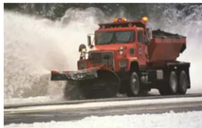
Automation of the snowplow vehicle is desired where a driver of the snowplow vehicle cannot see the guard rail covered with snow as shown in Fig. 1. The guard rail is often used as the reference of following road.
Driving under unseen guard rail situation may lead to a deadly accident if the vehicle hits the guard rail hidden under snow pile.
Research on automation of highway
maintenance vehicles has been initiated by the CALTRAN in California, USA. The autonomous highway management and construction technology (AHMCT) center at UC Davis is one of the leading research groups that conduct research on heavy duty field robotic vehicle projects. Several vehicles have already developed and utilized [1]. Similar research has also been conducted in Korea [2].
Automatic steering control of the vehicle is required for autonomous maneuvering along with GPS localization, GIS analysis, and sensor implementation.
Fig. 1. CALTRAN’s snowplow vehicle
The ultimate goal of this research is to develop the semi-autonomous snowplowing
vehicle that can follow the guard rail of the highway without collision. This requires accurate lateral control of the vehicle by maintaining a constant distance from the guard rail based on sensing information.
Active research on lateral control of the vehicles such as the ∞ control and the yaw rate feedback control has been presented [3-5]. Experimental studies of robust lateral control of a highway vehicle have been conducted [6,7]. Fuzzy control has been implemented for steering control [8,9].
In this paper, the feasibility of using four wheel steering control is investigated. As an extension of our previous research, a four wheeled vehicle is modelled and controlled.
The LQR control method is used to obtain optimal controllers’ gains for linearized model under load presence.
A neural network controller is introduced to compensate for disturbance rejection. Neural network is known as a powerful nonlinear controller and successful applications can be found [10-13].
Simulation studies are conducted for a Ford F-250 truck model and position tracking performances are compared under the virtual plowing condition.
Ⅱ. Four Wheel Steered Vehicle Dynamics
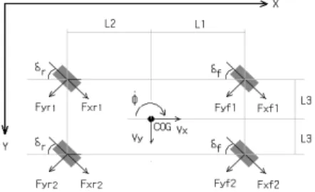
The vehicle is steered by both the front and the rear wheel [14].
Fig. 2. Model of 4 wheel steering vehicle X axis :
r yr r xr r yr r xr
f yf f xf f yf f xf x y
F F
F F
F F
F F
V V m
sin cos
sin cos
sin cos
sin cos
) (
2 2
1 1
2 2
1 1
.
Y axis
r yr r xr r yr r xr
f yf f xf f yf f xf y x
F F
F F
F F
F F
V V m
cos sin
cos sin
cos sin
cos sin
) (
2 2
1 1
2 2
1 1
.
Z axis
2 3 2 2 3 2
1 3 2 1 3 2
2 3 1 2 3 1
1 3 1 1 3 1 ..
) sin cos ( ) cos sin (
) sin cos ( ) cos sin (
) sin cos ( ) cos sin (
) sin cos ( ) cos sin (
yr r r xr
r r
yr r r xr
r r
yf f f xf
f f
yf f f xf
f f z
F L L F L L
F L L F L L
F L L F L L
F L L F L L I
(1) where is a total mass of the vehicle, is a yaw angle, is a steering angle of the front wheel, is a steering angle of the rear wheel, is the distance from the center of the front wheel to COG, is the distance from the center of the real wheel to COG,
is a velocity of the vehicle along direction,
is a velocity of the vehicle along direction, is a longitudinal force of the front wheel along direction, is a longitudinal force of the rear wheel along direction, is lateral force of the front wheel along direction, is a lateral force of the rear wheel along direction, is yaw moment of inertia along direction.
Slip angles are defined by
,
,
,
(2)
For simplicity, the vehicle is assumed to be symmetrical and its dynamics is considered as a bicycle model as shown in Fig. 3.
Fig. 3. Bicycle model of 4 wheel steered vehicle
The dynamic equations for the bicycle model are derived based on the references [14,15].
r yr f yf r xr f xf
x Vy F F F F
V
m( ) cos cos sin sin
.
.
r xr f xf f yf r yr
y Vx F F F F
V
m( ) cos cos sin sin
.
. (3)
r xr f xf r yr f yf
z LF LF LF LF
I 1 cos 2 cos 1 sin 2 cos
..
Slip angles are simplified as
,
(4)
where is a slip angle of the front wheel and is a slip angle of the rear wheel.
Lateral forces are defined as
, (5)
where and are cornering stiffness.
Under the assumption that the vehicle is moving at a constant velocity in longitudinal direction and the steer angle is small. A steering angle is considered as an control input, and a yaw angle and a lateral position
are outputs to be controlled.
Let and combining equations (3), (4), and (5) yields a MIMO system that has the state space representation as
(6)where
,
,
Ⅲ. LQR Control for Lateral Position
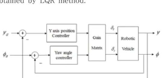
A LQR control block diagram for lateral position is shown in Fig. 4. The goal of the LQR control is to minimize the following objective function
∞ (7)where are the weighting matrices. values are selected based on trial and error process. The ultimate goal is to control the lateral position .
The lateral position error is formed as
(8)
The yaw angle is formed as
(9)
Those errors are multiplied by LQR controller gains. The controller outputs for the front steering and the rear steering are defined as
,
(10) where
,
are controller gains obtained by LQR method.
Fig. 4. Lateral control block diagram
For simplicity, we have the relationship
by not considering any dynamics of a steering actuator.
Ⅳ. Neural Network Control
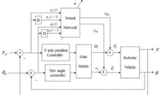
Here a neural network(NN) compensates for uncertainties by minimizing the errors defined in (10). The objective function is minimized in on-line fashion by adding compensating signal
from neural network to LQR controllers’ output [4].
A control inputs are defined by adding neural network outputs to (10) as
, (11)
where
are neural network outputs.
Fig. 5 shows the neural network control block diagram. At each sampling time, weights of neural network are updated to generate new compensating signals. The key issue here is how to implement on-line learning and control.
To achieve on-line control, certain computing power is required for parallel processing.
Fig. 5. Neural network control block diagram
A general feed-forward structure has an input layer, a hidden layer , and an output layer as shown in Fig. 6. For the control application, 4 input buffers, 6 hidden units and 2 output units are used.
Fig. 6. Neural network structure
For a nonlinear function at a hidden layer
and an output layer we have used the hyperbolic tangent function as
(12)
Since on-line learning and control is preferred, selecting training signals is very important. Typically, the bicycle model is a square MIMO system that two control inputs has to satisfy two different outputs simultaneously.
If is the system dynamics, equation (8), (10) and (11) can be represented as follows:
(13)
where
, and .
So the training signal of neural network as the sum of outputs of PD controllers is defined as
(14)
where .
The objective function is defined as
(15)
Differentiating (15) with respect to the weight w, we have
(16)
The update equation in back propagation algorithm is
∆
∆ (17) ∆ (18)
where is a learning rate and is a momentum coefficient.
Ⅴ. Simulation Studies
The following parameters of the vehicle are used for simulation studies.
Table 1. Parameters of 1985 Ford F-250
m Iz Cf, Cr L1 L2
5760 lb 2612.6
Kg
5860 (⋅sec)
810.2 (⋅sec)
9000 (lb/rad)
4082.3 (Kg/rad)
4.76 ft 1.45
m 6.35
ft 1.935
m Under the assumption of the constant longitudinal velocity, the state space representation of (6) becomes
(19)
LQR controller gains are selected from (19).
However, the robotic vehicle model described in (1) is used for the simulation model instead of using (19).
Different tracking responses of selecting gains as
and
are tested and their results are plotted in Fig. 7. We see that the large value of gives the good transient performance in the aspect of overshoot and settling time before 15 seconds. But when load (5000lb.ft/sec^2) is present after 15 seconds, tracking performance became the worst.
0 5 10 15 20 25 30
1.5 2 2.5 3 3.5 4
t (sec)
y (ft)
R=10 R=50 R=100
Fig. 7. Lateral control by LQR controllers We also altered the value of Q matrix, but
Q=I is found to be the best. We found that the value of Q matrix is more sensitive than that of R. Small change in Q results in bad tracking performances. Since the system is coupled, gain change affects tracking performances of both the position and the yaw angle.
Fig. 8 shows the tracking result when R=I, which shows a larger overshoot. The best tracking performance among several selections of R can be obtained when
and
. At that time, we have found the controller gains as
.
0 5 10 15 20 25 30
2 2.5 3 3.5 4 4.5
t (sec)
y (ft)
Fig. 8. Lateral position by LQR when R=I Next test is to compare results between two and four wheel steered vehicles under the same condition. We see here from Fig 9. that both cases show tracking errors when load is present. However, a four wheel steering vehicle shows less error although a two wheel steered vehicle shows no overshoot at a transient response.
0 5 10 15 20 25 30
1.8 2 2.2 2.4 2.6 2.8 3 3.2 3.4 3.6 3.8
t (sec)
y (ft)
Two wheel Drive Four W heel Drive
Fig. 9. Lateral position tracking results of two and four wheel steered vehicles
The plot explains that the system is much coupled so that optimized controller gains for
may not be optimal for both and .
3.1 Load is 1000⋅sec(138.2573N).
To minimize those tracking errors, the same simulation has been conducted by adding a neural network controller. For the neural network parameters, , are used and those values are optimized by trial and error basis. Fig.10 shows the lateral position tracking results for LQR control and neural network control.
0 5 10 15 20 25 30
2 2.2 2.4 2.6 2.8 3 3.2 3.4 3.6 3.8
t (sec )
y (ft)
NN R= 10
Fig. 10. Lateral position of LQR and NN
3.2 Load is 5000 ⋅sec(691.2864N)
Now the load has been increased to 5000
⋅sec after 15 seconds.
0 5 10 15 20 25 30
2 2.2 2.4 2.6 2.8 3 3.2 3.4 3.6 3.8
t (sec)
y (ft)
NN R=10
Fig. 11. Lateral position of LQR and NN
We see from Fig. 11 that the neural network controller outperforms in tracking
performance while the LQR controller cannot recover from an error deviation.
Ⅵ. Conclusion
This paper presents tracking control of lateral position of the autonomous four wheel steered vehicle. LQR controllers are designed based on a linearized model. The neural network controller is introduced to minimize tracking errors due to disturbance. Simulation studies show that the neural network controller outperforms LQR controller under present load conditions. A four wheel steered vehicle performs better than two wheel steered vehicle specially when load is present.
References
H
BIOGRAPHY
Seul Jung
Dr. Jung received B.S degree in Electrical &
Computer Engineering from Wayne State University, USA in 1988.
He received M.S and Ph. D. degree in both Electrical & Computer Engineering from University of California, Davis, 1991 and 1996, respectively. He is currently a professor at Mechatronics Engineering Department, Chungnam National University, Korea.
Research Interests : Intelligent mechatronics systems, creative robot design, human oriented robots, robot education.
Email : [email protected]
T. C. Hsia
Dr. T. C. Steve Hsia received the B.S. degree from National Taiwan University and the Ph.D.
degree from Purdue University, both in Electrical Engineering.
Dr. Hsia has been a Professor in the Department of Electrical and Computer Engineering at the University of California at Davis from 1965 to 2001, and a Professor Emeritus since 2001. Dr. Hsia has been a very active member in the IEEE Robotics and Automation Society. He has served as General Chair of IEEE ICRA'91. Dr. Hsia is an IEEE Fellow and the recipient of the IEEE Third Millennium Medal.
Email : [email protected]