The Impact of Macroeconomic Variables on the Profitability of Korean Ocean-Going Shipping Companies

(1)

DOI : http://dx.doi.org/10.5394/KINPR.2019.43.2.134

Myoung-Hee Kim*․†Ki-Hwan Lee

*,†Division of Shipping Management, Korea Maritime and Ocean University, Busan 49112, Republic of Korea

Abstract: The objective of this study was to establish whether global macroeconomic indicators affect the profitability of Korean shipping companies by using panel regression analysis. OROA (operating return on assets) and ROA (ratio of net profit to assets) were selected as proxy variables for profitability. OROA and ROA were used as dependent variables. The world GDP growth rate, interest rate, exchange rate, stock index, bunker price, freight, demand and supply of the world shipping market were set as independent variables.

The size of the firm was added to the control variable. For small-sized firms, OROA was not affect by macroeconomic indicators.

However, ROA was affected by variables such as interest rates, bunker prices, and size of firms. For medium-sized firms, OROA was affected by demand, supply, GDP, freight, and asset variables. However, macroeconomic indicators did not affect ROA. For large-sized firms, freight, GDP, and stock index (SCI; Shanghai Composite Index) have an effect on OROA. ROA was analyzed to be influenced by bunker price and SCI.

Key words : Profitability, Macroeconomic Variables, Korean Shipping Companies, Panel Regression Analysis, Company Size

†Corresponding author, [email protected] 051)410-4387

* [email protected] 051)410-4380

1. Introduction

In 1637, the collapse of the tulip bubble had shocked the Netherlands and Europe. As the history repeats, the shipping market bubble in 2007 and the financial crisis in 2008 have led to a long-term downturn in the shipping market.

Korea Line Corporation went into court receivership in 2011 and Pan Ocean Co., Ltd. files for court receivership in 2013. Hanjin Shipping Co., Ltd. went into bankruptcy in 2017. Since 2008, the number of companies closed due to corporate insolvency has increased significantly. Korean shipping companies are facing extreme difficulties, with the fierce competition in the global shipping market. As the shipping market is a derivative market, The performance of Korean shipping companies is expected to be affected by macroeconomic indicators in the global market. In this paper, we try to find macroeconomic variables that affect the profitability of Korean shipping companies. And the results of this study will help improve the profitability of Korean shipping companies.

There are very few papers considering various macroeconomic factors for the profitability of Korean shipping companies. Also, there are few papers that use panel data including both listed and unlisted companies.

Therefore in this study, we try to find macroeconomic variables that affect the profitability of Korean shipping companies using panel regression model. The variance of size among Korean shipping companies is very large. To solve size problems, the sample will be divided into several groups and analyzed by companies’ size. The deviation of firm size is minimized by this method. It helps to interpret the analysis results for each panel group. In addition, this study will analyze by panel regression model considering both the cross-sectional and time series factors. It is likely to be more useful in identifying the relationship between independent variables and dependent variables.

This study is organized as follows. A literature review will be conduct in section 2. In section 3, the data source and sample will be explained. And the empirical analysis and the result will be presented in section 4. The summary of this result and conclusion will be suggested in section 5.

2. Literature review

Drobetz et al.(2010) analyzed the macroeconomic risk factors that drive expected stock returns in the shipping industry. The sample consisted of 48 publicly-listed shipping companies. Monthly data from January 1999 to December 2007 were used to derive the results. The risk

(2)

factors of shipping companies were found to be non-systemic risk higher than systemic risk. the world stock market, currency fluctuations against the US$, changes in industrial production, and changes in the oil price are selected as macroeconomic variables that affect system risk.

El-Masry et al.(2010) examines the impact of financial risk and oil prices on stock returns of shipping companies in global markets. Financial risks include short-term interest rates, long-term interest rates and exchange rate.

143 shipping companies from 16 countries were selected as samples. The analysis period is from 1997 to 2005. The oil price affects returns of stock positively, but the other variables have no effect. However the result of sensitivity analysis by financial characteristics of companies is that stock returns is influenced negatively by the interest rates.

This paper explains that the exchange rate is not a risk factor because it is hedged by the corporation.

Lim and Lee(2014) analyzed the relationship between stock price of Korean shipping firms and macroeconomic variables. There is a cointegration relationship between the variables by the cointegration test. Thus, the relationship between stock prices index and macroeconomic variables was identified using the VECM model. Macroeconomic variables are exchange rate, interest rate, oil price, Baltic Dry Index, industry productivity. The result of this study is that industrial productivity before one period affects the stock index for shipping companies at the 5% significance level. At 10% significance level, oil price before one period affects stock price index.

Yang et al.(2015) analyzed whether exchange rate volatility affects a company 's profitability for a total of 55 Korean shipping companies during 2002-2013. Panel regression analysis was conducted before and after the global financial crisis. As a result, the exchange rate did not affect the profitability of the company before the financial crisis. However, after the financial crisis, the exchange rate has a negative impact on the profitability.

Park and An(2002) investigates how the variables affecting freight rates and freight rates affect firm stability and profitability. The study was conducted on Korean liner carriers. This study is analyzed whether supply and demand, shipping cost, characteristics of sipping company and other factors affect the freight rates for the liner carriers. As a result, supply and demand and characteristics of sipping company variables affect the freight rate. Also, it was analyzed that freight rate affects the stability and

profitability of shipping companies.

Ahn et al.(2017) studied about the estimation of elasticity of maritime transport demand using co-integration test.

The results of VECM(vector error correction model) analysis are as follows. When bunker price rise by 1%, the volume of the maritime transport declines by 0.15%. If the Clarkson Sea Index climbed 1%, the demand volume increased 0.04%. In addition, if global fleet increases by 1%, world marine trade volume will increase by 0.18%.

Kim(2013) analyzed the dynamic relationship between the Baltic Dry Freight Index (BDI) and international financial variables and China effect variables using VECM (Vector Error Correction Model). The result of this paper that Chinese imports, Dow Jones stock price and USD/JPY exchange rates have unidirectional effects on BDI. In recent years, In addition to there are some papers on the impact of China factor in maritime markets. Lu and Li(2009) and Mo(2006) investigated China effect in the world maritime market.

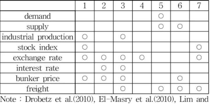
Table 1 Shows the macroeconomic variables related to the maritime market in the preceding study

Table 1 Macroeconomic variables of the literature review

1 2 3 4 5 6 7

demand ○

supply ○ ○

industrial production ○ ○

stock index ○ ○

exchange rate ○ ○ ○ ○ ○

interest rate ○ ○

bunker price ○ ○ ○ ○

freight ○ ○ ○ ○

Note : Drobetz et al.(2010), El-Masry et al.(2010), Lim and Lee(2014), Yang et al.(2015), Park and An(2002), Ahn et al.(2017) and Kim(2013) represent 1, 2, 3, 4, 5, 6 and 7.

Dependent variables as the financial performance of the company were selected as net profit, operating profit, and stock price return in previous studies. In addition, there are a few of studies to find macroeconomic variables that affect dependent variables as freight and demand.

In this paper, we will explore macroeconomic variables that affect the profitability of Korean shipping companies based on the review of previous studies mentioned above.

(3)

3. Data and sample

3.1 Data

In this study, unbalanced panel data of 46 companies are utilized as annual data from 2000 to 2017. OROA and ROA were selected as indicators of profitability, and two variables are dependent variables. ROA is the net profit to assets and OROA is the operating return on assets. The financial data of the 46 companies such as asset, sales, operating profit and net profit in DART (Data Analysis, Retrieval and Transfer System) of the Financial Supervisory Service.

Demand, Supply, GDP, SCI, FX, Libor, Oil, Freight, and Asset were set as independent variables. Demand is the world seaborne trade volume. Supply represents the tonnage of the world merchant fleets. GDP is the world GDP growth rate. SCI is a stock market index of all stocks that are traded at the Shanghai Stock Exchange. Index. FX is the won-dollar exchange rate. Libor is the 3month U$

Libor as an interest rate variable. Oil is the 180cst bunker prices, Singapore. Freight is the ClarkSea Index. Asset is a variable that indicates the size of the firm as total assets.

Data for macroeconomic indicators came from shipping intelligence of Clarkson, Shanghai Stock Exchange and Bank of Korea.

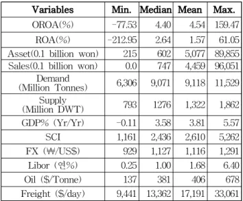
Table 2 Summary of variables

Variables Min. Median Mean Max.

OROA(%) -77.53 4.40 4.54 159.47 ROA(%) -212.95 2.64 1.57 61.05 Asset(0.1 billion won) 215 602 5,077 89,855 Sales(0.1 billion won) 0.0 747 4,459 96,051

Demand

(Million Tonnes) 6,306 9,071 9,118 11,529 Supply

(Million DWT) 793 1276 1,322 1,862 GDP% (Yr/Yr) -0.11 3.58 3.81 5.57

SCI 1,161 2,436 2,610 5,262

FX (₩/US$) 929 1,127 1,116 1,291

Libor (연%) 0.25 1.00 1.68 6.40

Oil ($/Tonne) 137 381 406 678

Freight ($/day) 9,441 13,362 17,191 33,061

3.2 Sample

In this study, we extracted companies operating in the sea freight water transport industry from DART (Data Analysis, Retrieval and Transfer System) of the Financial

Supervisory Service, as of March 2019. We excluded companies that were closed or M & A activities. The final analytical sample was selected for companies with at least 10 years of continuous historical financial data, including 2017. Forty-six companies that were able to obtain financial statements for 10 to 18 years in succession using DART were finally selected.

The size variation among Korean shipping companies is very large. The following Table 3 shows the mean, median, skewness and kurtosis of assets and sales for the last 10 years for 46 companies.

Table 3 Summary of quantile variables for grouping

Variables N Mean Median Skewness Kurto

sis Qantile 25% 50% 75%

Asset

(billion won) 46 569.7 68.1 3.9 16.2 35.2 68.1 440.3 Sales

(billion won) 46 467.1 86.2 4.3 19.7 26.8 86.2 234.7 ln(Asset) 46 7.1 6.5 0.8 -0.2 5.9 6.5 8.4 ln(Sales) 46 6.8 6.8 0.4 0.0 5.6 6.8 7.7

Both the assets and sales variables have a median value less than the average. This indicates that Korean shipping companies are composed of many small companies and a few large ones. Also skewness and kurtosis explain that the two variables do not follow the normal distribution.

When natural logarithm transformation is performed, the two variables follow a normal distribution. In the case of assets, the first quantile is 35.2 billion won, the second quantile is 68.1 billion won, and the third quantile is 440.3 billion won. In terms of sales, the first quantile is 26.8 billion won, the second quantile is 86.2 billion won, and the third quantile is 234.7 billion won.

3.3 Grouping

If the regression analysis is carried out without handling the size problem of the shipping companies the validity and reliability of the analysis result may be lacking. In order to solve the scale problem among Korean shipping companies, we perform panel regression analysis by classifying asset and sales variables into each 4 groups according to size.

(4)

4. Empirical analysis

4.1 Research model

The research model is as follows.

   

  



__{  } _ _{ } (1)

Here,  is a panel entity with 46 companies.  is the year variables from 2000 to 2017.  is the th independent variable and  is the number of independent variables. 

is the panel regression coefficient of the th independent variable.  is an individual characteristic of the panel that does not change with time. A panel regression model is a fixed effects model when  is considered as a parameter to be estimated. Assuming  is a random variable, it becomes a random effects model.   is the net error term not explained by the model.

4.2 Stationarity tests of time series

It is divided into each 4 groups by using quantiles based on assets and sales. Unit root tests were performed for panel regression analysis by each group. The Dickey-Fuller test for panel data checks for stochastic trends. The null hypothesis is that the series has a unit root. If p-value is less than 0.05 then no unit roots. A result of the tests, the asset variable was the not-stationary in three groups. For the three panel groups as the quantile 4 of asset and quantile 3, 4 of sales, the asset variable was required variable conversion. Taking the natural log, the asset variable is into a stationary time series.

4.3 Quantile regression analysis based on assets Table 4 is the results of the panel regression analysis of the quantile 1 group. In the quantile 1 group, p-value of F-statistic is over 0.05, the regression model is not significant at significance level 5% for OROA. However, regression model is significant for ROA. Libor and Bunker have negative effects on ROA. It means that the lower interest rate and bunker price impact on the corporate profits, positively. And the larger asset size leads to the better the profitability. ^ of the regression model for ROA is 18-19% in 1 quantile group. Both fixed and random

effect models are statistically significant. Random effects model is preferred by a result of Hausman test.

Table 4 Regression result for quantile 1 of asset (less than 35.15 billion won)

Data Unbalanced Panel: n=12, T=10-18, N=156 Dependent

variable OROA ROA

Fixed Random Fixed Random

R2 0.0539 0.0439 0.1963 0.1881

adj.R2 0.0466 0.0410 0.1699 0.1760 F-statistic 0.8552 0.7448 3.6657 3.7584 (p-value) (0.5669) (0.6673) (0.0003) (0.0002)

(Intercept) -28.3040 0.9094*

Demand -0.0057 -0.0058 0.0038 90.9450 Supply 0.0325 0.0320 -0.0413 0.0038

GDP 0.9004 0.8870 -1.2786 -0.0400

SCI -0.0005 -0.0008 -0.0005 -1.2695

FX 0.0340 0.0348 -0.0516 -0.0004

Libor 0.7780 0.9305 -2.7136* -0.0473* Oil -0.0074 -0.0086 -0.0202* -2.6052* Freight 0.0004 0.0004 -0.0003 -0.0179 　

Asset -0.0172 -0.0076 0.0256** -0.0003**

Hausman

Test chisq = 634.09, df = 9,

p-value < 2.2e-16 chisq = 1.4961, df = 9, p-value = 0.9972 Signif. codes: 0.01 ‘***’, 0.05 ‘**’, 0.1 ‘*’.

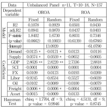
Table 5 is the results of the panel regression analysis of the quantile 2 group. It is shown that p-value of F-statistic is over 0.05, the regression models are not significant at significance level 5% in both OROA and ROA.

Table 5 Regression result for quantile 2 of asset (68.07-440.3 billion won)

variable OROA ROA

Fixed Random Fixed Random R2 0.1078 0.0929 0.0501 0.0430 adj.R2 0.0941 0.0870 0.0437 0.0403 F-statistic 1.8402 1.6730 0.8031 0.7346 (p-value) (0.0662) (0.1003) (0.6139) (0.6766)

(Intercept) 13.0920 -61.0790

Demand -0.0125 * -0.0121 * 0.0123 0.0116 Supply 0.0574 * 0.0559 * -0.0652 -0.0605 GDP 2.8626 ** 2.8220 ** 2.7336 2.8818 SCI -0.0001 0.0000 0.0001 0.0004 FX 0.0109 0.0123 0.0193 0.0269 Libor -0.9245 -0.8534 -0.5527 -0.6039 Oil -0.0102 -0.0089 -0.0100 -0.0079 Freight 0.0006 * 0.0006 * -0.0004 -0.0003 Asset -0.0015 -0.0009 0.0133 0.0090 Hausman

Test chisq = 1.7704, df = 9,

p-value = 0.9946 chisq = 4.5131, df = 9, p-value = 0.8745 Signif. codes: 0.01 ‘***’, 0.05 ‘**’, 0.1 ‘*’.

(5)

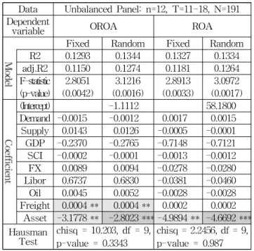
The result of an analysis for 3 quantile group of asset is Table 6. Freight is positive and Asset is negative for OROA. Only an asset variable effects on ROA, positively.

Table 6 Regression result for quantile 3 of asset (68.07-440.3 billion won)

variable OROA ROA

R2 0.1293 0.1344 0.1327 0.1334 adj.R2 0.1150 0.1274 0.1181 0.1264 F-statistic 2.8051 3.1216 2.8913 3.0972 (p-value) (0.0042) (0.0016) (0.0033) (0.0017)

(Intercept) -1.1112 58.1800

Demand -0.0015 -0.0012 0.0017 0.0015 Supply 0.0143 0.0126 -0.0005 -0.0001 GDP -0.2370 -0.2765 -0.7148 -0.7121 SCI -0.0002 -0.0001 -0.0013 -0.0012 FX 0.0089 0.0094 -0.0278 -0.0280 Libor 0.6737 0.6830 -0.0381 -0.0460 Oil 0.0045 0.0052 -0.0028 -0.0028 Freight 0.0004 ** 0.0004 ** 0.0002 0.0002

Asset -3.1778 ** -2.8023 *** -4.9894 ** -4.6692 ***

Hausman

Test chisq = 10.203, df = 9, p-value = 0.3343

chisq = 2.2456, df = 9, p-value = 0.987 Signif. codes: 0.01 ‘***’, 0.05 ‘**’, 0.1 ‘*’.

The results of an analysis for the quantile 4 group is shown in Table 7. Only Freight has a positive effect on OROA. And no variables have any effect on ROA.

Table 7 Regression result for quantile 4 of asset (over 440.3 billion won)

variable OROA ROA

R2 0.2007 0.1759 0.1303 0.1227

(Intercept) -11.5340 57.7570

Demand -0.0041 -0.0031 -0.0022 -0.0015 Supply 0.0146 0.0120 0.0002 -0.0026 GDP 1.0001 0.9521 2.0697 1.9996 SCI -0.0007 -0.0005 -0.0019 -0.0019 FX 0.0134 0.0170 -0.0354 -0.0358 Libor 0.0536 0.0559 -2.0026 -2.0090 Oil 0.0017 0.0043 -0.0069 -0.0065 Freight 0.0004 ** 0.0004 ** 0.0002 0.0002 Asset 0.8691 -0.1900 -0.2556 -0.1067 Hausman

Test chisq = 10.69, df = 9,

4.4 Quantile regression analysis based on sales Table 8 is the results of the panel regression analysis of the quantile 1 group. The model is not significant for OROA. Libor is having a negative effects on ROA. And an Asset has a positive effects on ROA. ^ of the regression model for ROA is 15-17% in 1 quantile group.

Table 8 Regression result for quantile 1 of sales (less than 26.8 billion won)

variable OROA ROA

R2 0.0404 0.0363 0.1486 0.1707

(Intercept) -53.4260 75.9760

Demand 0.0005 -0.0005 0.0072 0.0062 Supply 0.0065 0.0101 -0.0519 -0.0487 GDP 0.2243 0.3188 -1.4125 -1.3531 SCI -0.0001 -0.0003 0.0006 0.0004 FX 0.0362 0.0369 -0.0455 -0.0455 Libor 1.1415 1.2187 -2.6960 * -2.5639 *

Oil -0.0038 -0.0048 -0.0116 -0.0124 Freight 0.0004 0.0004 -0.0002 -0.0002

Asset -0.0037 -0.0008 0.0040 0.0065 **

Hausman

Table 9 Regression result for quantile 2 of sales (26.8-86.2 billion won)

variable OROA ROA

Fixed Random Fixed Random R2 0.1784 0.0807 0.0879 0.0603 adj.R2 0.1543 0.0753 0.0760 0.0562 F-statistic 3.0892 1.3470 1.3719 0.9850 (p-value) (0.0021) (0.2183) (0.2074) (0.4551)

(Intercept) 5.9519 -14.7350

Demand -0.0028 -0.0032 0.0092 0.0099 Supply 0.0148 0.0134 -0.0418 -0.0495 GDP -0.0275 0.0099 -0.8126 -0.8562 SCI 0.0002 0.0003 -0.0002 -0.0002

FX 0.0117 0.0091 0.0091 0.0030

Libor 1.0852 1.1743 0.5833 0.5191 Oil -0.0028 -0.0023 -0.0119 -0.0113 Freight 0.0001 0.0001 -0.0002 -0.0002 Asset -0.0089 *** -0.0020 -0.0075 0.0031 Hausman

Test chisq = 30.7, df = 9,

(6)

Table 9 is the results of the panel regression analysis of the quantile 2 group. It is shown that various variables such as Demand, Supply, GDP and Freight influence OROA. However, p-value of F-statistic is over 0.05. The regression model is not significant at significance level 5%.

The result of an analysis for 3 quantile group of asset is Table 10.

Table 10 Regression result for quantile 3 of sales (86.2-234.7 billion won)

variable OROA ROA

(Intercept) -6.7994 -35.7140

Demand -0.0110 ** -0.0097 * 0.0049 0.0048 Supply 0.0516 ** 0.0466 * -0.0334 -0.0325 GDP 2.4082 *** 2.2520 ** 2.4205 2.4713 SCI -0.0006 -0.0003 -0.0001 0.0000

FX 0.0150 0.0169 0.0184 0.0205

Libor -0.8154 -0.6930 -0.2444 -0.2599 Oil -0.0013 0.0012 0.0119 0.0130 Freight 0.0007 *** 0.0007 *** 0.0000 0.0000 Asset 0.0000 0.0001 0.0003 0.0000 Hausman

Test chisq = 54.298, df = 9, p-value = 1.657e-08

Demand is having a negative impact in OROA. However, Supply, GDP, Freight have negative effects on OROA. It means that the increase in GDP and freight lead to a positive operating profits of companies. This can be easily understood. However, in the case of demand and supply, the result is not easily recognized. The unit of measure of a Demand variable is million tonnes. It can be interpreted that when 1 million tonnes of cargo volume grows, the OROA of the company decreases by 0.0110%. In other words, it does not need to give a big meaning. Supply variable can also be interpreted similarly to Demand because the measurement unit is large. There are no macroeconomic variables affecting ROA.

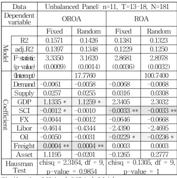
The results of the panel regression analysis for the quantile 4 group is shown in Table 11. GDP and Freight have a positive effect on OROA. And SCI has a negative effect on OROA. In case of OROA, the random effects model is preferred for this group by Hausman test. SCI is not significant variable in random effect model.

Table 11 Regression result for quantile 4 of sales (over 234.7 billion won)

variable OROA ROA

(Intercept) 17.7760 100.7400

Demand -0.0061 -0.0058 -0.0068 -0.0068 Supply 0.0257 0.0255 0.0316 0.0308 GDP 1.1335 * 1.1259 * 2.3405 2.3032

SCI -0.0012 * -0.0010 -0.0033 ** -0.0033 **

FX -0.0044 -0.0012 -0.0646 -0.0668 Libor -0.4614 -0.4344 -2.4390 -2.4695 Oil -0.0050 -0.0031 -0.0229 * -0.0236 * Freight 0.0004 ** 0.0004 ** 0.0003 0.0003

Asset 1.1195 -0.0201 -0.1265 0.2777 Hausman

chisq = 0.1305, df = 9, p-value = 1 Signif. codes: 0.01 ‘***’, 0.05 ‘**’, 0.1 ‘*’.

SCI and Oil have a negative effect on ROA. When bunker price increase, it effect on shipping cost. Thus, the rise in bunker price leads to a decline in profitability of shipping companies. It is necessary to study whether the oil price variable responds to net profit without responding to operating profit. SCI. The rise in SCI has been shown to have a negative impact on OROA and ROA. This is similar to the result of the Mo(2006)’ research. Mo(2006) explained that the result was due to multi-collinearity problems.

Competition between Korea and China shipping companies is becoming more intense, due to China factor. Profitability is likely to decline despite the growth of the Chinese economy, as domestic shipping companies are not able to maintain a competitive advantage in the global market.

5. Conclusion

In this study, we tried to grasp macroeconomic variables affecting profitability of Korean shipping companies. We selected OROA (operating return on assets) and ROA (ratio of net profit to assets) as proxy variables for profitability.

OROA and ROA were used as dependent variables. The world GDP growth rate, interest rate, exchange rate, stock index, oil price, demand and supply of the world shipping market were set as independent variables. The size of the firm was added to the control variable.

(7)

The results of this study are as follows.

For 1 quantile group, macroeconomic indicators do not affect POA. However, Libor and Bunker are showing negative effects on ROA. Asset is shown to have a positive impact. For 2 quantile group, there are no macroeconomic indicators affecting POA and ROA. Only asset variable has a negative effect on ROA. For 3 quantile group, supply, GDP and Freight affect on POA, positively. However POA is negatively affected by Demand. Asset only has a negative effect on ROA. Lastly, in case of 4 quantile group, GDP and Freight have a positive impact on POA. However, SCI is found to have a negative effect on POA. SCI and Bunker price have negative effects on ROA.

The contribution of this study is as follows.

This paper is examined whether global macroeconomic indicators affect the profitability of Korean shipping companies. Empirical analysis was performed using a panel regression analysis. The variation of the firm size within shipping companies is very large. Asset and sales were analyzed by setting subgroups by size. It helps to interpret the analysis results as some errors due to corporate deviations are minimized. In addition, this study was analyzed by panel regression model considering both the cross-sectional and time series factors. It is likely to be more helpful in identifying the relationship between independent variables and dependent variables.

The results of this study is that the macroeconomic variables affecting the profitability of firms are different depending on the size of firms. It will contribute to the risk management of the corporation. In addition, it will be useful in the decision-making process of the various stakeholders of the Korean shipping company, depending on the size.

The limitations of this study are as follows.

It is not easy to acquire time series data of companies that can be acquired before the financial crisis. Therefore, in this study, we do not perform panel regression analysis by grouping before and after the global financial crisis.

However, in future research, it is necessary to perform panel regression analysis by grouping them before and after the global financial crisis. Before and after the global financial crisis, we need to see whether the macroeconomic variables that affect profitability of Korean shipping companies are different.

There are some companies with extreme data. This is not data coding mistake, but it is characteristics of these shipping companies. However if the size of the firm holding the outlier data is large, it may affect the overall model

result. Therefore we used the data as a sample. In addition, it is necessary to remove the companies with outlier and then fit the model and discuss the results.

References

[1] Ahn, Y. G., Kim, J. H. and Lee, M. K.(2017), “The Estimation of Elasticity of Maritime Transport Demand Using Co-Integration Test”, Korea logistic review, Vol.

2, No. 6, pp. 211-219.

[2] Drobetz, W., Schilling, D. and Tegtmeier, L.(2010),

“Common risk factors in the returns of shipping stocks”, Maritime Policy & Management, Vol. 37, No.

2, pp. 93-120.

[3] El-Masry, A. A., Olugbode, M. and Pointon, J.(2010),

“The exposure of shipping firms’ stock returns to financial risks and oil prices: a global perspective”, Maritime Policy & Management, Vol. 37, No. 5, pp.

453-473.

[4] Han, C. H.(2004), “China Effect in the Tanker Shipping Market”, Ocean&Fisheries(Monthly Report), Vol. 232, pp. 26-35.

[5] Kim, C. B.(2013), “Dynamic Causality among International Financial Variables, China Effect, and Shipping Business Cycle after the Global Financial Crisis”, The Journal of shipping and logistics, Vol. 78, pp. 575-588.

[6] Lee, S. Y.(2015), “The Relationship between Working Capital Management and Profitability : evidence from Korean Shipping Industry”, Journal of navigation and port research, Vol. 39, No. 3, pp. 261-266.

[7] Lim, J. K.(2004), “China Effect in the Shipping Market”, Ocean&Fisheries(Monthly Report), Vol. 232, pp. 6-7.

[8] Lozinskaia, A., Merikas, A., Merika, A. and Penikas, H.(2017), “Determinants of the probability of default : the case of the internationally listed shipping corporations”, Maritime Policy & Management, Vol. 44, No. 7, pp. 837-858.

[9] Lu, F. and Li, Y.(2009), “The China factor in recent global commodity price and shipping freight volatilities”, China Economic Journal,Vol. 2, No. 3, pp. 351-377.

[10] Mo, S. W.(2006), “China Effect in the Dry Bulk Shipping Market”, The Journal of shipping and logistics, Vol. 49, pp. 1-19.

[11] Nam, H. J. and An, Y. H.(2017), “Default Risk and Firm Value of Shipping & Logistics Firms in Korea”, The Asian Journal of Shipping and Logistics, Vol. 33, No. 2, pp. 61-65.

(8)

[12] Park, H. G. and An, K. M.(2002), “A Study on the Determinant and the Stabilization Scheme of Liner Freight Rates”, Shipping and Studies : Theory and Practice, Spring, pp. 47-82.

[13] Shin, S. S.(2004), “China Effect in the Dry Bulk Shipping Market”, Ocean&Fisheries(Monthly Report), Vol. 232, pp. 18-25.

[14] Yang, H. J., Lee, K. H. and Kim, M. H.(2015), “An Empirical Study of the Impact of Exchange Rate Fluctuation on Profitability of Korean Ocean-Going Shipping Companies”, The journal of Shipping and Logistics, Vol. 31, No. 2, pp. 407-425.

[15] Yin, H., Chen, Z. and Xiao, Y.(2019), “Risk perception affecting the performance of shipping companies: the moderating effect of China and Korea”, Maritime Policy & Management, Vol. 46, No. 3, pp. 295-308.

Received 1 April 2019 Revised 9 April 2019 Accepted 25 April 2019