Korean Chemical Engineering Research

204 PISSN 0304-128X, EISSN 2233-9558

Water + N-Methyldiethanolamine (MDEA), Water + 2-Amino-2-Methyl-1-Propanol (AMP), MDEA + AMP, Water+ MDEA + AMP 계의 밀도와 과잉부피 측정 및 상관

나재석 · 민병무* · 박영철* · 문종호* · 전동혁* · 이종섭* · 신헌용^† 서울과학기술대학교 화공생명공학과

01811 서울시 노원구 공릉로 232

*한국에너지기술연구원 온실가스연구실 34129 대전광역시 유성구 가정로 152

(2017년 8월 25일 접수, 2017년 10월 20일 수정본 접수, 2017년 10월 25일 채택)

Measurement and Correlation of Densities and Excess Volumes for Water + N-Methyldiethanolamine (MDEA), Water + 2-Amino-2-Methyl-1-Propanol (AMP),

MDEA + AMP and Water + MDEA +AMP systems

Jaeseok Na, Byoung-Moo Min*, Young Cheol Park*, Jong-Ho Moon*, Dong Hyuk Chun*, Jong-Seop Lee* and Hun Yong Shin^† Department of Chemical and Biomolecular Engineering, Seoul National University of Science & Technology, 232 Gongneung-ro,

Nowon-gu, Seoul, 01811, Korea

*Climate Change Research Division, Korea Institute of Energy Research, 152 Gajeong-ro, Yuseong-gu, Daejeon, 34129, Korea (Received 25 August 2017; Received in revised form 20 October 2017; accepted 25 October 2017)

요 약

Water+N-Methyldiethanolamine (MDEA), Water+2-Amino-2-Methyl-1-Propanol (AMP), MDEA+AMP의 이성분계, Water+MDEA+AMP의 삼성분계에서 밀도를 Anton Paar DMA4500 밀도계를 이용하여 303.15 K에서 333.15 K의 온 도범위에서 10 K 간격으로 혼합물의 전체 조성에서 측정하였다. 과잉부피 실험값은 실험적으로 측정된 밀도결과로부 터 얻어졌고 Redlich-Kister-Muggianu 식으로 상관하였다. 이성분계로부터 얻은 매개변수를 이용하여 삼성분계에 대한 계산을 수행하였다. 삼성분계의 계산에는 하나의 추가적인 매개변수를 필요로 한다. 검토한 모든 이성분계와 삼성분계는 측정된 조건에서 과잉부피가 음의 값을 가지므로 완전히 섞임을 알 수 있다.

Abstract − In this study, densities of water + N-Methyldiethanolamine (MDEA), Water + 2-Amino-2-Methyl-1-Propa- nol (AMP), MDEA + AMP binary systems and Water+MDEA+AMP ternary system were measured over the full range of composition at temperatures from 303.15 K to 333.15 K by using an Anton Paar digital vibrating tube densimeter (DMA4500). The experimental excess volumes have been obtained from the experimental density results and have been fitted using the Redlich-Kister-Muggianu expression. The parameters obtained from the binary excess volume data were used for the correlation of ternary system with one additional ternary parameter for each isotherm. All investigated binary and ternary systems are completely miscible, because the values of excess volume are negative under the examined conditions.

Key words: Density, Excess volume, Water, N-methyldiethanolamine, 2-amino-2-methyl-1-propanol

1. 서 론

지구온난화로 인한 환경 변화에 대응하기 위하여 온실가스 감축 이 의무화되어 이를 이행하기 위한 방법이 필요하다. 이산화탄소 배출을 저감하기 위하여 다양한 온실가스 회수 공정이 연구되고 있

으며 연소 후 회수법, 연소 전 회수법 및 순산소 연소법이 알려져 있다[1-3]. 연소 후 회수법은 연소 후 가스에서 흡수제를 이용하여 이산화탄소를 흡수한 뒤 이를 다시 탈거부에서 분리하여 순수한 이 산화탄소만을 포집할 수 있으며, 이 과정에서 재생된 흡수제 또한 재사용 할 수 있다. 흡수공정에 사용하는 흡수제로 알칸올아민이 대표적으로 알려져 있다. 알칸올아민은 이산화탄소에 높은 친화도 를 가지고 있어 연소 후 공정에서 흡수제로 사용할 수 있다. 대표적 인 알칸올아민으로는 Monoethanolamine (MEA), Diethanolamine (DEA), N-Methyldiethanolamine (MDEA), Diisopropanolamine (DIPA), 2-Amino-2-Methyl-1-Propanol (AMP) 등이 있다[4]. 기존 연소 후

†To whom correspondence should be addressed.

E-mail: [email protected]

This is an Open-Access article distributed under the terms of the Creative Com- mons Attribution Non-Commercial License (http://creativecommons.org/licenses/by- nc/3.0) which permits unrestricted non-commercial use, distribution, and reproduc- tion in any medium, provided the original work is properly cited.

공정에서는 단일 알칸올아민를 중점으로 연구가 되었으나 최근 연 구에선 알칸올아민 혼합물의 활용에 대해서 연구가 진행되고 있다 [5-7]. 알칸올아민 혼합물을 사용할 때 단일 알칸올아민에 비해 더 좋은 흡수능과 낮은 재생에너지 등의 좋은 물리적 특성을 얻을 수 있다. 공정모사에는 물성을 정확히 측정하는 것이 중요하며 물성은 물질의 고유한 특성으로 실험을 통해 측정할 필요가 있다. 특히, 습 식 흡수 공정에서 대량의 흡수제가 순환될 때 유속이 낮아질 수 있 으므로 이를 정확히 계산할 필요가 있고 이 중 밀도는 활동도 계수 모델의 계산에 이용할 수 있다[8,9]. 본 연구는 새로운 이산화탄소의 연소 후 포집공정에 적용할 수 있는 알칸올아민 흡수제 혼합제의 밀도와 과잉부피의 측정을 통해 공정 설계의 기초 데이터를 제공하 고자 한다. N-Methyldiethanolamine과 2-Amino-2-Methtyl-1-Propanol 은 기존에 사용되던 Monoethanolamine에 비해 낮은 반응열과 재 생에너지를 갖는 이점이 있다[10,11]. N-Methyldiethanolamine 수 용액과 2-amino-2-methyl-1-propanol 밀도와 과잉부피에 대해선 일부 데이터가 문헌에 보고되었다[12-14]. 그러나 MDEA+AMP의 이성 분계와 Water + MDEA + AMP의 삼성분계에 대해선 부피데이터의 측정결과가 보고되지 않고 있다. 본 연구에서는 Water + MDEA, Water + AMP, MDEA + AMP의 이성분계와 Water + MDEA + AMP 삼성분계의 밀도와 과잉부피를 측정하였다. 측정된 밀도데이터로 부터 얻어진 과잉부피는 Redlich-Kister-Muggianu 식으로 상관하 였다[15].

2. 실 험

N-methyldiethanolamine은 순도가 99% 이상인 Sigma-Aldrich의 시약을 사용하였고, 2-Amino-2-Methyl-1-Propanol은 순도가 99%

이상인 Acros Organics의 시약을 사용하였다. 증류수는 순도가 99.99% 이상인 Samchun Chemical의 시약을 사용하였다. 모든 시

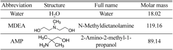
약은 추가적인 정제과정 없이 사용되었다. 실험이 진행되는 동안 밀도 측정을 통하여 순도를 확인하였다. 사용된 화학성분들의 구조 식, 분자량을 Table 1에 나타내었다.

2-2. 장치 및 실험과정

이성분, 삼성분 혼합물 시료는 디지털미량저울(Ohaus Co.

PAG214)을 이용하여 목표하는 몰분율에 해당하는 질량만큼의 순 수시약을 20 ml 유리 시약병에 넣은 뒤 혼합하여 제조하였다. 디지 털미량저울의 정확도는 ±1.0×10⁻⁴ g 이며 이 실험에서 시료의 몰분 율의 측정 불확도는 0.0002 이하이다. 이 실험에서 Anton Paar DMA4500 밀도계를 이용하여 밀도를 측정하였다. 밀도계의 정확 도는 ±0.05 kg m⁻³이며 증류수와 공기로 밀도계를 보정하였다. 밀 도계에 준비된 시료를 3 ml PP 실린지를 이용하여 밀도계의 튜브에 주입한 후 평형상태에 도달하였을 때 밀도를 측정하였다. 측정한 온도는 303.15 K에서 333.15 K 사이에서 10 K 간격으로 측정하였다.

측정된 온도의 정확도는 ±0.01 K이다. 각 시료의 측정 후, 튜브는 물과 아세톤으로 세척하였다.

3. 결과 및 고찰

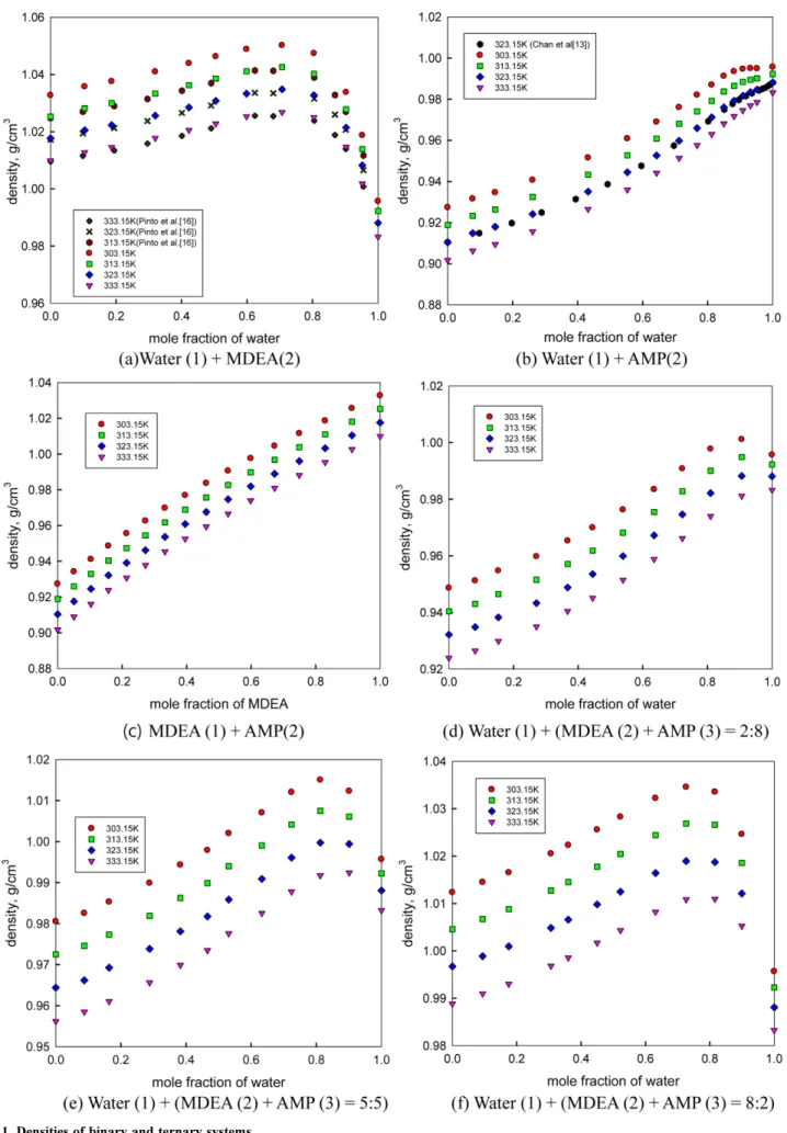
Water(1)+MDEA(2) 이성분계의 303.15 K에서 333.15 K까지의 측정한 밀도는 Table 2와 Fig. 1(a)에 나타내었다. 313.15 K, 323.15 K, 333.15 K에서 문헌[16]의 밀도데이터와 비교하였으며 잘 일치하는 것을 확인하였다. Water (1)+MDEA (2)의 밀도는 물의 조성 x1= 0.7 부분까지 증가하다 순수한 물의 밀도에 수렴하였다. Water(1) + AMP(2) 이성분계의 303.15 K에서 333.15 K까지의 측정된 밀도는 Table 3와 Fig. 1(b)에 나타내었다. 밀도는 물의 조성 x₁= 0.93까지 증가하다가 감소하여 순수한 물의 밀도에 수렴하였다. 323.15 K에서 문헌의 밀도와 비교하였을 때 잘 일치하였다[13]. MDEA (1) + AMP (2) 이성분계의 303.15 K에서 333.15 K까지의 측정된 밀도는 Table 4 와 Fig. 1(c)에 나타내었다. 밀도는 MDEA의 조성이 증가함에 따라 증가하였다. 흡수제 혼합물중의 흡수제의 질량비를 일정하게 두어, Water (1) + (MDEA (2) + AMP (3) = 2:8) 삼성분계의 303.15 K에서 333.15 K까지의 측정된 밀도는 Table 5와 Fig. 1(d)에 나타내었다.

밀도는 물의 조성 x₁= 0.9까지 증가하다가 순수한 물의 밀도로 수 렴하였다. Water (1) + (MDEA (2) + AMP (3) = 5:5) 삼성분계의 303.15 K에서 333.15 K까지의 측정된 밀도는 Table 6와 Fig. 1(e)에 나타 Table 1. Molar masses of pure components

Abbreviation Structure Full name Molar mass

Water H₂O Water 18.02

MDEA N-Methyldietanolamine 119.16

AMP 2-Amino-2-methyl-1-

propanol 89.14

Table 2. Experimental Densities and Excess volumes of the Water (1) + MDEA (2) system

x₁ Density(g/cm³) Excess volume(cm³/mol)

303.15 K 313.15 K 323.15 K 333.15 K 303.15 K 313.15 K 323.15 K 333.15 K

0.0000 1.0327 1.0253 1.0176 1.0099 0.0000 0.0000 0.0000 0.0000

0.1043 1.0358 1.0282 1.0205 1.0128 -0.3784 -0.3608 -0.3575 -0.3542

0.1867 1.0376 1.0300 1.0223 1.0146 -0.5788 -0.5574 -0.5500 -0.5435

0.3197 1.0410 1.0333 1.0256 1.0178 -0.8746 -0.8475 -0.8324 -0.8179

0.4226 1.0439 1.0362 1.0284 1.0205 -1.0681 -1.0355 -1.0132 -0.9913

0.5047 1.0463 1.0386 1.0308 1.0228 -1.1829 -1.1466 -1.1200 -1.0937

0.5985 1.0488 1.0411 1.0333 1.0253 -1.2603 -1.2205 -1.1896 -1.1600

0.7071 1.0502 1.0426 1.0348 1.0268 -1.2267 -1.1859 -1.1515 -1.1184

0.8043 1.0474 1.0402 1.0327 1.0250 -1.0346 -0.9996 -0.9697 -0.9413

0.9025 1.0338 1.0278 1.0214 1.0147 -0.6137 -0.5952 -0.5803 -0.5662

0.9520 1.0187 1.0139 1.0082 1.0018 -0.3134 -0.3062 -0.2950 -0.2785

1.0000 0.9957 0.9923 0.9881 0.9832 0.0000 0.0000 0.0000 0.0000

Fig. 1. Densities of binary and ternary systems.

내었다. 밀도는 x₁= 0.8까지 증가하다가 순수한 물의 밀도에 수렴 하였다. Water (1)+(MDEA (2)+AMP (3)=8:2) 삼성분계의 303.15 K 에서 333.15 K까지의 측정된 밀도는 Table 7와 Fig. 1(f)에 나타내 었다. 밀도는 x1= 0.7까지 증가하다가 순수한 물의 밀도로 수렴하 였다. 측정된 모든 이성분계, 삼성분계에서 온도가 증가할수록 밀 도는 감소하였다.

측정된 실험값으로 과잉부피 V^E를 계산하였으며 이 때 V^E는 식 (1)으로 계산하였다.

(1)

ρ는 혼합물의 밀도, ρ_i는 순수성분 i의 밀도, M_i는 순수성분 i의 분 자량이다.

Water (1) + MDEA (2) 이성분계와 Water (1) + AMP (2) 이성분

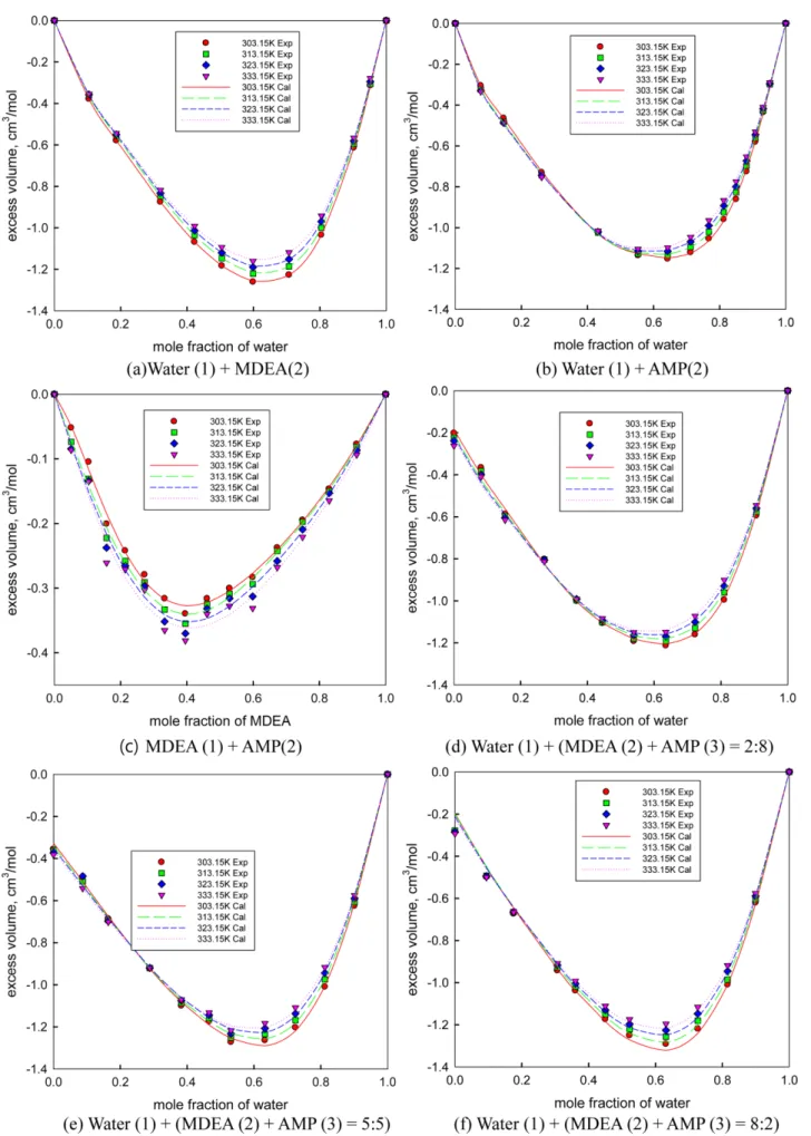
계의 303.15 K에서 333.15 K까지의 과잉부피는 각각 Table 2,3와 Fig. 2(a), (b)에 나타내었다. 두 계에서 과잉부피는 x1= 0.6 근처에서 최저점을 가진다. Water (1) + MDEA (2) 계에선 모든 조성에서 온 도가 증가할수록 과잉부피가 감소하였으나 Water (1) + AMP (2)계 에선 x₁= 0부터 0.45까지는 온도가 증가할수록 과잉부피는 증가하 였고 그 이후로는 온도가 증가할수록 과잉부피는 감소하였다.

MDEA (1) + AMP (2) 이성분계의 303.15 K에서 333.15 K까지의 과잉부피는 Table 4과 Fig. 2(c)에 나타내었다. 과잉부피는 x1= 0.4 근처에서 최저점을 가지며 온도가 증가할수록 과잉부피는 증가하 였다. Water (1) + (MDEA (2) + AMP (3)) 삼성분계에서는 다른 질 량비율로 혼합된 이성분 혼합물들과 물을 혼합한 혼합물로 측정한 결과로 이를 303.15 K에서 333.15 K까지의 측정한 과잉부피는 각각 Table 5-7와 Fig. 2(d)-(f)에 나타내었다. Water (1) + (MDEA (2) + AMP (3) = 2:8)에서는 과잉부피는 x1= 0.6에서 최저점을 가지며 x1= 0부터 V^E x_iM_i

---ρ

n i 1=

∑

i

---

n i 1=

∑

–

=

Table 3. Experimental Densities and Excess volumes of the Water (1) + AMP (2) system

x₁ Density(g/cm³) Excess volume(cm³/mol)

303.15 K 313.15 K 323.15 K 333.15 K 303.15 K 313.15 K 323.15 K 333.15 K

0.0000 0.9274 0.9188 0.9104 0.9018 0.0000 0.0000 0.0000 0.0000

0.0771 0.9316 0.9233 0.9148 0.9063 -0.3048 -0.3239 -0.3299 -0.3339

0.1462 0.9346 0.9263 0.9179 0.9094 -0.4638 -0.4817 -0.4867 -0.4877

0.2614 0.9407 0.9325 0.9241 0.9157 -0.7294 -0.7429 -0.7443 -0.7530

0.4319 0.9515 0.9433 0.9350 0.9265 -1.0218 -1.0246 -1.0207 -1.0155

0.5529 0.9609 0.9528 0.9445 0.9360 -1.1360 -1.1276 -1.1157 -1.1045

0.6427 0.9690 0.9609 0.9526 0.9442 -1.1529 -1.1344 -1.1157 -1.0978

0.7121 0.9761 0.9680 0.9598 0.9514 -1.1209 -1.0947 -1.0690 -1.0466

0.7674 0.9821 0.9741 0.9659 0.9576 -1.0532 -1.0199 -0.9901 -0.9644

0.8123 0.9870 0.9792 0.9712 0.9630 -0.9590 -0.9240 -0.8928 -0.8665

0.8497 0.9912 0.9837 0.9760 0.9681 -0.8611 -0.8277 -0.7989 -0.7748

0.8812 0.9935 0.9865 0.9792 0.9717 -0.7248 -0.6968 -0.6726 -0.6529

0.9083 0.9947 0.9884 0.9817 0.9746 -0.5799 -0.5609 -0.5443 -0.5305

0.9316 0.9950 0.9895 0.9834 0.9769 -0.4358 -0.4264 -0.4177 -0.4100

0.9519 0.9949 0.9901 0.9846 0.9785 -0.3003 -0.2987 -0.2946 -0.2891

1.0000 0.9957 0.9923 0.9881 0.9832 0.0000 0.0000 0.0000 0.0000

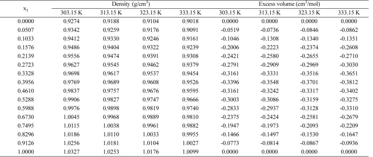
Table 4. Experimental Densities and Excess volumes of the MDEA (1) + AMP (2) system

x₁ Density(g/cm³) Excess volume (cm³/mol)

303.15 K 313.15 K 323.15 K 333.15 K 303.15 K 313.15 K 323.15 K 333.15 K

0.0000 0.9274 0.9188 0.9104 0.9018 0.0000 0.0000 0.0000 0.0000

0.0507 0.9342 0.9259 0.9176 0.9091 -0.0519 -0.0736 -0.0846 -0.0862

0.1033 0.9412 0.9330 0.9246 0.9161 -0.1046 -0.1308 -0.1340 -0.1351

0.1576 0.9486 0.9404 0.9322 0.9239 -0.2006 -0.2223 -0.2374 -0.2608

0.2139 0.9556 0.9474 0.9391 0.9308 -0.2421 -0.2580 -0.2655 -0.2710

0.2723 0.9627 0.9545 0.9462 0.9379 -0.2791 -0.2909 -0.2969 -0.3030

0.3328 0.9698 0.9617 0.9537 0.9454 -0.3161 -0.3331 -0.3516 -0.3651

0.3956 0.9769 0.9689 0.9608 0.9526 -0.3396 -0.3548 -0.3701 -0.3812

0.4610 0.9837 0.9757 0.9676 0.9595 -0.3161 -0.3242 -0.3317 -0.3402

0.5288 0.9906 0.9827 0.9747 0.9666 -0.3003 -0.3086 -0.3159 -0.3275

0.5988 0.9976 0.9898 0.9819 0.9740 -0.2833 -0.2937 -0.3128 -0.3310

0.6730 1.0045 0.9968 0.9889 0.9810 -0.2375 -0.2424 -0.2581 -0.2679

0.7495 1.0115 1.0038 0.9961 0.9882 -0.1947 -0.1973 -0.2093 -0.2209

0.8296 1.0186 1.0110 1.0033 0.9955 -0.1466 -0.1497 -0.1530 -0.1647

0.9126 1.0256 1.0181 1.0104 1.0027 -0.0773 -0.0814 -0.0867 -0.0936

1.0000 1.0327 1.0253 1.0176 1.0099 0.0000 0.0000 0.0000 0.0000

0.3까지는 온도가 증가할수록 과잉부피는 증가하였고 x1= 0.3부터 1까지는 감소하였다. Water (1) + (MDEA (2) + AMP (3) = 5:5) 삼 성분계에서는 과잉부피는 x1= 0.6에서 최저점을 가지며 x1= 0부터 0.2까지는 온도가 증가할수록 과잉부피는 증가하였고 x1= 0.2부터 1에서는 감소하였다. Water (1) + (MDEA (2) + AMP (3) = 8:2) 삼 성분계에서는 x₁= 0.6에서 최저점을 가지며 x₁= 0부터 0.1까지는 온도가 증가할수록 증가하였고 x1= 0.1부터 1에서는 감소하였다.

모든 계에서 과잉부피는 음의 값을 가지며 조성의 변화에 따라 한 개의 최저점을 갖는 포물선 형태를 나타내었다. 삼성분계에서 물의 조성 x1= 0인 조건에서 측정된 시료는 순수 성분이 아닌 설정된 일 정 조성의 이성분 흡수제 혼합물이므로 계산된 과잉부피가 0이 아 닌 값을 갖는다. 이성분계와 삼성분계의 과잉부피는 Redlich- Kister-Muggianu[15] 식을 이용하여 상관하였다. 이성분계에서 식 (2)으로 상관하였다.

Table 5. Experimental Densities and Excess volumes of Water (1) + (MDEA (2) + AMP (3) = 2:8 weight fraction) system

x₁ x₂ Density (g/cm³) Excess volume (cm³/mol)

303.15 K 313.15 K 323.15 K 333.15 K 303.15 K 313.15 K 323.15 K 333.15 K

0.0000 0.1576 0.9486 0.9404 0.9322 0.9239 -0.2018 -0.2235 -0.2387 -0.2621

0.0812 0.1448 0.9512 0.9430 0.9348 0.9265 -0.3653 -0.3823 -0.3983 -0.4097

0.1531 0.1334 0.9547 0.9465 0.9382 0.9299 -0.5875 -0.5970 -0.6056 -0.6153

0.2710 0.1149 0.9598 0.9516 0.9433 0.9350 -0.8018 -0.8037 -0.8058 -0.8135

0.3675 0.0997 0.9653 0.9571 0.9488 0.9405 -1.0014 -0.9975 -0.9917 -0.9905

0.4448 0.0875 0.9700 0.9618 0.9536 0.9451 -1.1067 -1.1017 -1.0925 -1.0834

0.5389 0.0726 0.9763 0.9682 0.9599 0.9515 -1.1919 -1.1794 -1.1641 -1.1497

0.6350 0.0575 0.9835 0.9755 0.9672 0.9588 -1.2129 -1.1924 -1.1696 -1.1486

0.7226 0.0437 0.9908 0.9828 0.9746 0.9662 -1.1607 -1.1300 -1.1012 -1.0728

0.8100 0.0299 0.9978 0.9901 0.9821 0.9740 -0.9954 -0.9607 -0.9295 -0.9012

0.9063 0.0148 1.0012 0.9949 0.9882 0.9812 -0.5948 -0.5762 -0.5596 -0.5450

1.0000 0.0000 0.9957 0.9923 0.9881 0.9832 0.0000 0.0000 0.0000 0.0000

Table 6. Experimental Densities and Excess volumes of Water (1) + (MDEA (2) + AMP (3)= 5:5 weight fraction) system

x₁ x₂ Density (g/cm³) Excess volume (cm³/mol)

303.15 K 313.15 K 323.15 K 333.15 K 303.15 K 313.15 K 323.15 K 333.15 K

0.0000 0.4279 0.9806 0.9725 0.9644 0.9562 -0.3554 -0.3650 -0.3729 -0.3821

0.0875 0.3905 0.9826 0.9746 0.9662 0.9585 -0.4964 -0.5085 -0.4840 -0.5419

0.1640 0.3578 0.9853 0.9773 0.9693 0.9611 -0.6860 -0.6930 -0.6980 -0.7020

0.2881 0.3047 0.9899 0.9819 0.9739 0.9657 -0.9228 -0.9203 -0.9202 -0.9198

0.3827 0.2642 0.9943 0.9863 0.9781 0.9699 -1.0997 -1.0863 -1.0756 -1.0701

0.4658 0.2286 0.9979 0.9899 0.9818 0.9735 -1.1746 -1.1578 -1.1442 -1.1320

0.5313 0.2006 1.0020 0.9940 0.9859 0.9776 -1.2726 -1.2513 -1.2327 -1.2174

0.6330 0.1570 1.0071 0.9991 0.9909 0.9826 -1.2641 -1.2345 -1.2077 -1.1829

0.7241 0.1181 1.0120 1.0042 0.9961 0.9878 -1.2028 -1.1683 -1.1371 -1.1079

0.8124 0.0803 1.0150 1.0075 0.9997 0.9918 -1.0096 -0.9745 -0.9437 -0.9167

0.9011 0.0423 1.0123 1.0061 0.9994 0.9924 -0.6255 -0.6063 -0.5900 -0.5752

1.0000 0.0000 0.9957 0.9923 0.9881 0.9832 0.0000 0.0000 0.0000 0.0000

Table 7. Experimental Densities and Excess volumes of Water (1) + (MDEA (2) + AMP (3)= 8:2 weight fraction) system

x₁ x₂ Density (g/cm³) Excess volume (cm³/mol)

303.15 K 313.15 K 323.15 K 333.15 K 303.15 K 313.15 K 323.15 K 333.15 K

0.0000 0.7495 1.0123 1.0046 0.9967 0.9888 -0.2813 -0.2785 -0.2850 -0.2933

0.0942 0.6789 1.0145 1.0067 0.9989 0.9910 -0.4990 -0.4929 -0.4951 -0.4999

0.1754 0.6181 1.0165 1.0088 1.0009 0.9930 -0.6728 -0.6652 -0.6646 -0.6663

0.3064 0.5199 1.0205 1.0127 1.0048 0.9968 -0.9423 -0.9275 -0.9179 -0.9084

0.3603 0.4794 1.0223 1.0145 1.0066 0.9986 -1.0376 -1.0189 -1.0050 -0.9926

0.4501 0.4122 1.0256 1.0178 1.0098 1.0017 -1.1736 -1.1499 -1.1298 -1.1109

0.5225 0.3579 1.0283 1.0205 1.0125 1.0043 -1.2503 -1.2215 -1.1971 -1.1737

0.6313 0.2763 1.0322 1.0244 1.0164 1.0082 -1.2915 -1.2564 -1.2260 -1.1957

0.7265 0.2050 1.0346 1.0269 1.0190 1.0108 -1.2186 -1.1807 -1.1473 -1.1159

0.8157 0.1381 1.0335 1.0266 1.0187 1.0109 -1.0091 -0.9864 -0.9457 -0.9184

0.8993 0.0755 1.0246 1.0186 1.0121 1.0053 -0.6203 -0.6035 -0.5892 -0.5759

1.0000 0.0000 0.9957 0.9923 0.9881 0.9832 0.0000 0.0000 0.0000 0.0000

Fig. 2. Excess volumes of binary and ternary systems.

+ (2) 삼성분계에서 식 (3)으로 상관하였다

+

+

+ + (3)

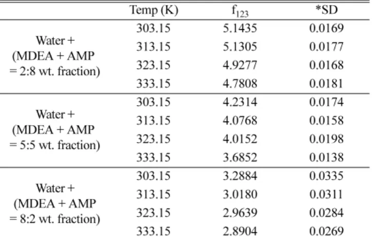
매개변수 A, B, C는 이성분의 과잉부피 실험결과로부터 얻어진 값 이며 Table 8에 나타내었다. 매개변수 A는 성분 1과 성분 2 혼합물, 매개변수 B는 성분 2와 성분 3 혼합물에서, 매개변수 C는 성분 1과 성분 3 혼합물의 과잉부피를 계산하여 얻어진 변수이다. 삼성분계 에서는 삼성분 실험데이터로부터 추가적인 매개변수 f123을 추산하 여 Table 9에 나타내었고 계산 결과를 Fig. 2(d)-(f)에 나타내었다.

과잉부피 계산의 표준편차 Sd는 식 (4)로 구하였다.

(4)

N은 같은 온도조건에서의 실험값의 수이며 n은 Redlich-Kister- Muggianu 식에서 사용한 변수의 수이다. 실험데이터의 최적화로부 터 얻은 표준편차는 Table 8, 9에 나타내었다.

과잉부피의 변화는 쌍극자-쌍극자 힘, 분산력, 수소결합을 포함 하는 분자간 상호작용과 분자의 크기, 구조, 입체장애 등 분자의 기 하학적 특성이 작용한다. 모든 계에서 과잉부피가 음의 값을 나타 내는데 이는 다른 분자간에 상호작용이 강하여 같은 조건의 이상용 액에 비해 부피가 작다는 것을 의미한다. 즉, 혼합에 의해 부피가 감소하게 된다. 물, MDEA, AMP 모두 -OH기를 가지고 있어 수소 결합을 형성할 수 있고 이는 강한 분자간 상호작용으로서 과잉부피 가 음의 값을 갖는 주요 요인이 된다. 또한, 물이 포함된 계에서 과 잉부피의 최저점은 물의 조성이 높은 영역에서 형성되는데 이는 물 분자의 3차원 격자구조에 용질이 수용되는 것에 기인한 것으로 판 단 된다[17,18].

4. 결 론

Water + MDEA, Water + AMP, MDEA + AMP 이성분계에 대한 밀도를 전체 조성범위에서 측정하였으며, 흡수제 혼합물(MDEA + AMP)의 질량비를 일정하게 둔 3가지 조건에서 Water + MDEA + AMP 삼성분계의 밀도를 303.15 K에서 333.15 K까지의 온도범위 에서 측정하였다. 모든 계에서 과잉부피가 음의 값을 가지며 이로 부터 각 혼합물이 혼합되는 것을 확인할 수 있다. 측정된 실험값들은 Redlich-Kister-Muggianu 식으로 상관하였고 실험데이터와 잘 일 치하는 것을 볼 수 있다. 삼성분계는 흡수제 혼합물의 질량조성을 일정하게 두고 실험하였으며, 삼성분의 과잉부피 계산에서는 하나의 추가적인 매개변수를 추가하였다.

감 사

이 논문은 한국에너지기술평가원과 산업통상자원부의 지원으로 수행된 과제(No. 20152020201130)의 연구결과입니다.

사용기호

A_i, B_i, C_i : parameters of Redlich-Kister-Muggianu equation f₁₂₃ : additional parameter of Redlich-Kister-Muggianu equation V^E=x₁x₂[A₀+A₁(x₁–x₂) A+ ₂(x₁–x₂)²+A₃(x₁–x₂)³

A₄(x₁–x₂)⁴+A₅(x₁–x₂)⁵]

V^E=x₁x₂[A₀+A₁(x₁–x₂) A+ ₂(x₁–x₂)²+A₃(x₁–x₂)³ A₄(x₁–x₂)⁴+A₅(x₁–x₂)⁵]

+ x₂x₃[B₀+B₁(x₂–x₃) B+ ₂(x₂–x₃)²+B₃(x₂–x₃)³ B₄(x₂–x₃)⁴+B₅(x₂–x₃)⁵]

+ x₁x₃[C₀+C₁(x₁–x₃) C+ 2(x₁–x₃)²+C₃(x₁–x₃)³ C₄(x₁–x₃)⁴+C₅(x₁–x₃)⁵] x₁x₂x₃f₁₂₃

S_d

∑

N n–

( )

---

1/2

=

Table 8. Redlich-Kister-Muggianu Model Parameters for binary systems

Temp. (K) A₀ A₁ A₂ A₃ A₄ A₅ *SD

Water + MDEA

303.15 -4.7102 -2.3386 -1.3407 -0.7147 0.1118 2.4154 0.0020

313.15 -4.5657 -2.2441 -1.2351 -0.6989 0.0867 2.1903 0.0020

323.15 -4.4607 -2.1189 -1.1473 -0.6935 -0.0408 2.1027 0.0034

333.15 -4.3565 -2.0043 -1.1000 -0.6544 -0.1094 1.9783 0.0070

Water + AMP

303.15 -4.4334 -1.3686 -1.1172 -3.9485 -0.6897 5.1846 0.0120

313.15 -4.4105 -1.2939 -0.9066 -3.1823 -1.1062 4.4961 0.0091

323.15 -4.3699 -1.2514 -0.7111 -2.5229 -1.3818 3.7764 0.0077

333.15 -4.3352 -1.1657 -0.6336 -2.0552 -1.4782 3.1802 0.0087

MDEA + AMP

303.15 -1.2526 0.5507 -0.1463 -0.4874 0.5569 -0.2029 0.0088

313.15 -1.2975 0.6152 -0.0561 -0.5948 0.1314 0.1778 0.0101

323.15 -1.3499 0.5923 -0.0834 -0.5444 0.1344 0.2538 0.0147

333.15 -1.3965 0.5268 -0.1436 -0.1738 0.1363 -0.1977 0.0195

Table 9. Redlich-Kister-Muggianu Model Parameters for ternary systems

Temp (K) f₁₂₃ *SD

Water + (MDEA + AMP

= 2:8 wt. fraction)

303.15 5.1435 0.0169

313.15 5.1305 0.0177

323.15 4.9277 0.0168

333.15 4.7808 0.0181

Water + (MDEA + AMP

= 5:5 wt. fraction)

303.15 4.2314 0.0174

313.15 4.0768 0.0158

323.15 4.0152 0.0198

333.15 3.6852 0.0138

Water + (MDEA + AMP

= 8:2 wt. fraction)

303.15 3.2884 0.0335

313.15 3.0180 0.0311

323.15 2.9639 0.0284

333.15 2.8904 0.0269

*SD = Standard Deviation

for ternary system

M_i : molecular weight of components i n : numbers of parameters

N : numbers of experimental data V^E : excess volume

S_d : standard deviation

x_i : mole fraction of components i ρ : density of mixture

ρ_i : density of pure components i

References

1. Wall, T. F., “Combustion Processes for Carbon Capture,” Proc.

Combust. Inst, 31, 31-47(2007).

2. Yang, H., Xu, Z., Fan, M., Gupta, R., Wall, T. F., Slimane, R. B., Bland, A. E. and Wright, I., “Progress in Carbon Dioxide Sepa- ration and Capture: A Review,” J. Environ. Sci, 20, 14-27(2008).

3. Saha, A. K., Bandyopadhyay, S. S., Saju, P. and Biswas, A. K.,

“Selective Removal of Hydrogen Sulfide from Gases Containing Hydrogen Sulfide and Carbon Dioxide by Absorption into Aqueous Solutions of 2-amino-2-methyl-1-propanol,” Ind. Eng. Chem. Res., 32, 3051-3055(1993).

4. Kohl, A. L. and Nielsen, R. B., Gas Purification, 5th ed, Gulf Publishing, Houston, TX(1997).

5. Bruggink, S., Beyad, Y., Luo, W., MeliánCabrer, I., Puxty, G. and Feron, P., “CO₂ Absorption Into Aqueous Amine Blended Solu- tions Containing Monoethanolamine (MEA), N,N-dimethyletha- nolamine (DMEA), N,N-diethylethanolamine (DEEA) and 2-amino- 2-methyl-1-propanol (AMP) for Post Combustion Capture Pro- cesses,” Chem. Eng. Sci., 126, 446-454(2015).

6. Muchan, P., Saiwan, C., Narku-Tetteh, J., Idem, R., Supap, T. and Tontiwachwuthikul, P., “Screening Tests of Aqueous Alkanolamine Solutions Based on Primary, Secondary, and Tertiary Structure for Blended Aqueous Amine Solution Selection in Post Combus- tion CO₂ Capture,” Chem. Eng. Sci., 170, 574-582(2017).

7. Gervasia, J., Duboisa, L. and Thomasa, D., “Screening Tests of New Hybrid Solvents for the Post-combustion CO₂ Capture Pro- cess by Chemical Absorption,” Energy Procedia, 63, 1854-1862 (2014).

8. Austgen, D. M., Rochelle, G. T., Peng, X. and Chen, C.-C., “Model of Vapor-liquid Equilibria for Aqueous Acid Gas-alkanolamine Systems Using the Electrolyte-NRTL Equation,” Ind. Eng. Chem.

Res., 28(7), 1060-1073(1989).

9. Voutsas, E., Vrachnos, A. and Magoulas, K., “Measurement and

Thermodynamic Modeling of the Phase Equilibrium of Aqueous N-methyldiethanolamine Solutions,” Fluid Phase Equilibria, 224, 193-197(2004).

10. Mandal, B. P., Kundu, M. and Bandyopadhyay, S. S., “Density and Viscosity of Aqueous Solutions of (N-Methyldiethanolamine + Monoethanolamine), (N-Methyldiethanolamine + Diethanolamine), (2-Amino-2-methyl-1-propanol + Monoethanolamine), and (2- Amino-2-methyl-1-propanol + Diethanolamine),” J. Chem. Eng.

Data, 48, 703-707(2003).

11. Chen, C.-C. and Song, Y., “Generalized Electrolyte-NRTL Model for Mixed-solvent Electrolyte Systems,” AIChE J., 50, 1928-1941 (2004).

12. Shokouhi, M., Jalili, A. H., Samani, F. and Hosseini-Jenab, M.,

“Experimental Investigation of the Density and Viscosity of CO₂- loaded Aqueous Alkanolamine Solutions,” Fluid Phase Equilibria, 404, 96-108(2015).

13. Chan, C., Maham, Y., Mather, A. E. and Mathonat, C., “Densities and Volumetric Properties of the Aqueous Solutions of 2-amino- 2-methyl-1-propanol,n-butyldiethanolamine Andn-propylethanol- amine at Temperatures from 298.15 to 353.15 K,” Fluid Phase Equilibria 198, 239-250(2002).

14. Sobrinoa, M., Concepción, E. I., Gómez-Hernández, Á., Martín, M. C. and Segovia, J. J., “Viscosity and Density Measurements of Aqueous Amines at High Pressures: MDEA-water and MEA- water Mixtures for CO₂ Capture,” J. Chem. Thermodynamics, 98, 231-241(2016).

15. Redlich, O. and Kister, A. T., “Algebraic Representation of Thermo- dynamic Properties and the Classification of Solutions,” Ind. Eng.

Chem., 40, 345-348(1948).

16. Pinto, D. D. D., Monteiro, J. G. M.-S., Johnsen, B., Svendsen, H.

F. and Knuutila, H., “Density Measurements and Modelling of Loaded and Unloadedaqueous Solutions of MDEA (N-methyldieth- anolamine), DMEA(N,N-dimethylethanolamine), DEEA (diethy- lethanolamine) and MAPA(N-methyl-1,3-diaminopropane),”

International Journal of Greenhouse Gas Control, 25, 173-185 (2014).

17. Rafiee, H. R. and Frouzesh, F., “Volumetric Properties for Binary and Ternary Mixtures of Allyl Alcohol, 1,3-dichloro-2-propanol and 1-ethyl-3-methyl Imidazolium Ethyl Sulfate [Emim][EtSO₄] from T = 298.15 to 318.15 K at Ambient Pressure,” Thermochimica Acta, 611, 36-46(2015).

18. Chowdhury, F. I., Khan, M. A. R., Saleh, M. A. and Akhtar, S.,

“Volumetric Properties of Some Water + monoalkanolamine Sys- tems Between 303.15 and 323.15 K,” J. Mol. Liq, 182, 7-13(2013).